Modelling a jet fan that is not aligned with the FDS grid: louvers vs a rotated GEOM fan

TL;DR

• FDS makes an aligned jet fan easy: an OBST, two HVAC VENTs and a duct. A fan rotated in plan has no native OBST equivalent.
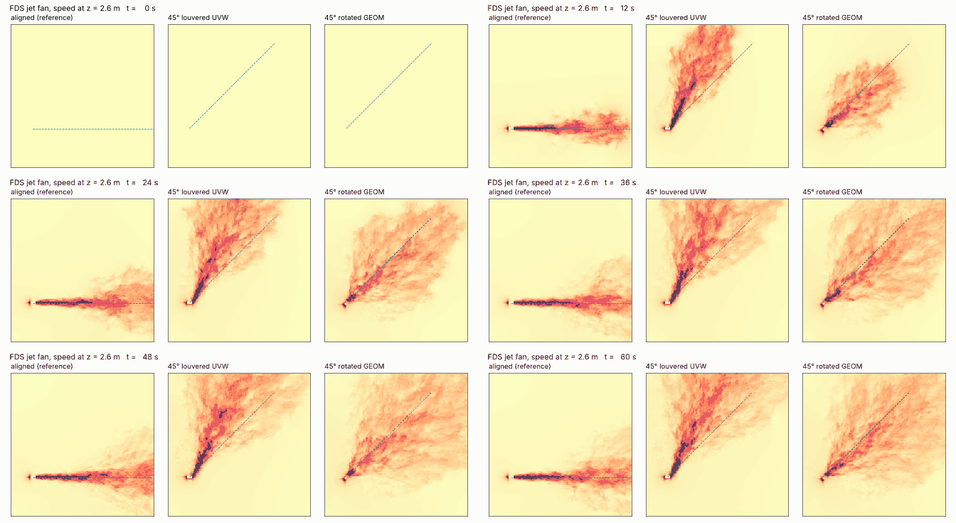
• The usual workaround, a louvered outlet (UVW on the HVAC VENT), did not produce a 45° jet in our runs: the jet ended up at ≈62° (17° too far) and its exit speed and thrust were 41 % too high. Widening the outlet by 1/cos θ fixes the thrust and reduces the error (≈55.5°), but the direction is still wrong.
• A truly rotated fan — a GEOM box turned with &MOVE, with HVAC nodes on its faces (FDS 6.11.0 or newer) — kept the direction within ≈5° (≈40–43°).
• It is not free: GEOM fans ran 3.4–3.7× slower than the aligned fan (≈€17–18 vs ≈€6 for 60 s on 32 cores), and with the same 2.0 m³/s they gave a 24–26 % weaker jet core 1 m from the outlet — check exit velocity and throw before trusting them.
• If all your fans are parallel, the cheapest exact answer is still to rotate the model, not the fan, so the fans line up with the grid.

Why this question keeps coming up

Car parks, tunnels and warehouses are rarely drawn on a neat grid. Jet fans follow the ramps, the column lines and the exits, so in a typical impulse-ventilation layout several fans sit at 20–60° to the axes of the FDS mesh. FDS is a Cartesian, block-structured LES code: every OBST is snapped to the grid and every VENT must lie on a cell face, so a fan “box” cannot simply be rotated.

The FDS User’s Guide gives the classic recipe for a free-standing jet fan (an obstruction with two HVAC vents, see the example jet_fan.fds) and suggests UVW on the outlet vent to give the flow a direction that is not along an axis. On the FDS forum the developers confirm that, for a jet that is not orthogonal to the grid, putting a tangential component on the discharge vent is the practical way, and recommend grid sensitivity runs. FDS 6.11 added a second option: HVAC nodes can now sit on the faces of an unstructured GEOM, and a GEOM can be rotated with &MOVE.

We wanted numbers, not opinions: the same fan, aligned and at 45°, modelled three ways, run on FDS on cloudHPC. If you are new to the aligned recipe, start from our earlier post on the jet fan model in FDS; for why jet fans matter in car parks, see CO extraction and CFD in car parks.

Results at a glance

Case	How the fan is modelled	FDS needed	Jet direction (intended)	Exit speed / thrust from the inputs	Peak speed at 1 m / 10 m	Wall time per simulated s (32 cores)	Cost of the 60 s run
A00	aligned OBST + 2 HVAC VENTs (reference)	any	0.0° (0°)	12.5 m/s / 30.1 N	9.8 / 4.2 m/s	40 s	€5.95
G00	GEOM box, not rotated, HVAC nodes on faces, ULMAT	≥ 6.11.0	0.0° (0°)	12.5 m/s / 30.1 N	7.5 / 3.5 m/s	134 s	€16.69
L45	aligned box, louvered outlet UVW=(cos45°, sin45°, 0)	≥ 6.7	61.8° (45°)	17.7 m/s / 42.6 N	13.8 / 4.3 m/s	55 s	€7.55
C45	as L45, fan body and vents widened 0.4 → 0.6 m (≈ 1/cos θ, grid-snapped)	≥ 6.7	55.5° (45°)	11.8 m/s / 28.4 N	10.7 / 3.9 m/s	36 s	€5.46
G45	GEOM box rotated 45° with &MOVE, HVAC nodes on faces, ULMAT	≥ 6.11.0	39.9° (45°)	12.5 m/s / 30.1 N	7.3 / 3.0 m/s	145 s	€18.12

Jet direction: median over 4–12 m of the speed-weighted direction of the time-averaged 3D velocity field (the horizontal slice at fan-axis height gives 64.1°, 57.0° and 42.8° for L45, C45 and G45). Peak speed: maximum time-averaged speed at distance r from the outlet centre — in the vertical plane through the axis for the 0° fans, over a vertical half-cylinder (±60° around the intended direction) for the 45° fans. All cases delivered exactly 2.0 m³/s through the HVAC duct.

How the runs were set up

• Solver: FDS 6.11.1 (Intel build with HYPRE), LES with default Deardorff turbulence model, isothermal (20 °C), no fire.
• Domain: an open-sided car-park slab, 32 × 26 m, floor and ceiling walls, 3.0 m clear height, OPEN vents on all four sides.
• Mesh: uniform 0.1 m cells, 2.5 M cells in 32 meshes (8 × 4 of 40 × 65 × 30 cells), one MPI process per mesh.
• Fan: 1.0 m long body, 0.4 × 0.4 m inlet and outlet, centre at (4.0, 7.0, 2.6) m, so the top of the fan is 0.2 m below the ceiling. HVAC duct with VOLUME_FLOW=2.0 m³/s → 12.5 m/s on the 0.16 m² outlet, ≈30 N of thrust. The outlet is 4 cells across, one cell more than the minimum Alshroof found necessary for an impulse jet fan in FDS.
• Outputs: 200 probes on the intended jet axis from 0.1 m to 20 m in front of the outlet (time-averaged U, V, W and speed), rotated with the fan through &MOVE; transverse probe lines at 1, 2, 5, 10, 15 and 20 m; a horizontal slice through the axis; a vertical slice through the axis (PBY for the aligned fans, a 3D slice box cut along the rotated axis in post-processing for the 45° fans, since FDS slices are always grid-aligned).
• Statistics: 60 s simulated, averages over 20–60 s. The probe 10 m along the axis (z = 2.85 m) changed by 1–6 % between the 20–40 s and 40–60 s windows in the cases where the jet passes there (A00 3.92 → 3.98 m/s, G00 3.21 → 3.38 m/s, G45 2.16 → 2.13 m/s).
• Instances: cloudHPC hypercore, 32 vCPU (physical cores), regular (non-preemptible) instances so the timings are clean.

The three ways to model the fan

Aligned fan (A00) — the textbook recipe

&OBST ID='FAN BODY', XB=3.5,4.5,6.8,7.2,2.4,2.8 /
&VENT ID='FAN IN',  XB=3.5,3.5,6.8,7.2,2.4,2.8, SURF_ID='HVAC' /
&VENT ID='FAN OUT', XB=4.5,4.5,6.8,7.2,2.4,2.8, SURF_ID='HVAC' /
&HVAC ID='FAN IN',  TYPE_ID='NODE', DUCT_ID='JET FAN', VENT_ID='FAN IN' /
&HVAC ID='FAN OUT', TYPE_ID='NODE', DUCT_ID='JET FAN', VENT_ID='FAN OUT' /
&HVAC ID='JET FAN', TYPE_ID='DUCT', NODE_ID='FAN IN','FAN OUT', VOLUME_FLOW=2.0, AREA=0.16 /

Louvered outlet (L45, C45) — works in any FDS from 6.7

Same block, with a direction on the outlet vent:

&VENT ID='FAN OUT', XB=4.5,4.5,6.8,7.2,2.4,2.8, SURF_ID='HVAC', UVW=0.707107,0.707107,0.0 /

FDS keeps the normal velocity at Q/A and adds the tangential component needed to point the flow along UVW. The exit speed therefore becomes (Q/A)/cos θ: at 45° the jet leaves at 17.7 m/s instead of 12.5 m/s and carries 41 % more momentum than the real fan. In C45 we compensated by widening the fan body and both vents by about 1/cos θ (0.4 → 0.6 m, the nearest grid-compatible width; the duct AREA stays 0.16 m²), which gives 11.8 m/s and 28.4 N — within 6 % of the real fan.

Rotated GEOM fan (G00, G45) — FDS 6.11.0 or newer

&PRES SOLVER='ULMAT' /
&SURF ID='FAN IN SURF',  NODE_ID='FAN IN' /
&SURF ID='FAN OUT SURF', NODE_ID='FAN OUT' /
&MOVE ID='FAN ROT', X0=4.0, Y0=7.0, Z0=2.6, AXIS=0,0,1, ROTATION_ANGLE=45.0 /
&GEOM ID='FAN BODY', XB=3.5,4.5,6.8,7.2,2.4,2.8,
      SURF_ID6='FAN IN SURF','FAN OUT SURF','INERT','INERT','INERT','INERT', MOVE_ID='FAN ROT' /
&HVAC ID='FAN IN',  TYPE_ID='NODE', DUCT_ID='JET FAN', GEOM=T /
&HVAC ID='FAN OUT', TYPE_ID='NODE', DUCT_ID='JET FAN', GEOM=T /
&HVAC ID='JET FAN', TYPE_ID='DUCT', NODE_ID='FAN IN','FAN OUT', VOLUME_FLOW=2.0, AREA=0.16 /

The SURF that carries NODE_ID must have no other boundary condition, and GEOM=T tells the HVAC node to look for a GEOM face instead of a VENT. SURF_ID6 lists the faces as −x, +x, −y, +y, −z, +z, so the first face is the intake and the second the outlet. The same &MOVE can rotate DEVC lines (MOVE_ID on a DEVC with POINTS), which is how our probes follow the fan.

Case 1 — where does the jet actually go?

Case	Intended	Measured, 3D field (median 4–12 m)	Measured, horizontal slice at z = 2.6 m (median 4–14 m)	Error
A00	0°	0° (symmetry plane)	0.04°	0°
G00	0°	0° (symmetry plane)	0.13°	0°
L45	45°	61.8°	64.1°	+17° to +19°
C45	45°	55.5°	57.0°	+10.5° to +12°
G45	45°	39.9°	42.8°	−2° to −5°

What we learned

• The louvered outlet turns the jet too far. The FDS forum warns that on a coarse grid the tangential component you prescribe may not be reached; here the opposite happened. The jet leaves the vent at roughly the intended 45° (44° at 1 m) but keeps bending over the first 4–5 m and settles at 60–62°, 17–19° off. We did not run the grid study needed to explain why — treat it as a measured fact for this set-up, not a law.
• Fixing the momentum (C45) also reduces the over-turning, but 10.5–12° is still large: across a 40 m car park it moves the jet by about 8 m.
• The rotated GEOM fan points where you put it, within the 2–5° scatter of a turbulent jet measured on a 0.1 m grid.

Case 2 — how far does the jet throw?

Case	Peak speed at r = 1 m	5 m	10 m	Distance where the peak drops below 3 m/s
A00	9.8 m/s	8.0 m/s	4.2 m/s	14.0 m
G00	7.5 m/s	6.0 m/s	3.5 m/s	12.0 m
L45	13.8 m/s	7.2 m/s	4.3 m/s	> 11.5 m (beyond the 3D slice)
C45	10.7 m/s	5.3 m/s	3.9 m/s	> 11.5 m (beyond the 3D slice)
G45	7.3 m/s	4.0 m/s	2.96 m/s	9.0 m (not monotonic: 3.09 m/s again at 10.5 m)

What we learned

• The aligned fan keeps a straight core for about 8 m at fan height before attaching to the ceiling. All three 45° models lose their core much sooner, rise towards the ceiling within 2–5 m and spread much faster.
• The axial DEVC line is a trap for misaligned fans: on the intended axis the louvered jets read under 0.5 m/s at 5 m (L45) simply because the jet is somewhere else. Always check the direction before reading probes on an assumed axis.
• GEOM fans are weaker near the outlet even when not rotated: G00 gives 7.5 m/s at 1 m against 9.8 m/s for the identical aligned OBST fan, with the same 2.0 m³/s through the duct. Less exit momentum for the same flow means a shorter throw (12 m vs 14 m to drop below 3 m/s). Rotating the GEOM fan by 45° costs another 3 m of throw on a 0.1 m grid.
• In a real design, calibrate: put a DEVC with QUANTITY='VELOCITY' 0.5–1 m in front of each fan model and compare its peak with the aligned reference (or the manufacturer’s throw data) before using the fan layout for smoke clearance.

Run times and costs

Run	cloudHPC instance	Time steps	Mean time step	Solver wall time	Wall time per simulated s	Billed vCPU-h	Cost
A00	hypercore 32, regular	10,683	5.6 ms	39.7 min	40 s	27.1	€5.95
G00	hypercore 32, regular	17,121	3.5 ms	134.4 min	134 s	75.9	€16.69
L45	hypercore 32, regular	14,662	4.1 ms	55.3 min	55 s	34.3	€7.55
C45	hypercore 32, regular	9,849	6.1 ms	36.4 min	36 s	24.8	€5.46
G45	hypercore 32, regular	20,521	2.9 ms	145.0 min	145 s	82.4	€18.12
Total						244.4	€53.77

Billed time includes boot, end-of-run detection and the upload of results (about 8–11 minutes per run). The sizing runs used to plan the series cost another €12.64.

Two things drive the cost of the GEOM fans:

1. The pressure solver. Any GEOM switches FDS to the global unstructured UGLMAT solver (HYPRE). On a 2 s test of G45, it spent 70 % of the run time in the pressure solve at 0.81 s per step; with &PRES SOLVER='ULMAT' / (a direct solve per mesh, fine for meshes under ~150,000 cells) the share dropped to 7 % and the step to 0.49 s — 1.7× faster. All production GEOM runs used ULMAT. The 7 % is an average over the 32 MPI processes: on the meshes that hold the fan the pressure solve still takes up to about half of the time, and the other processes spend roughly half of theirs waiting for them. Smaller meshes around the fan would balance the load better.
2. The time step. Small cut cells at the fan faces keep the time step 38–48 % smaller than in the aligned case (2.9–3.5 ms vs 5.6 ms), even when the fan is not rotated.

The louvered L45 runs 39 % longer than A00 (27 % higher cost) for a simpler reason: its jet leaves at 17.7 m/s, so the CFL limit gives a smaller time step.

Failures we met on cloudHPC (and what they mean)

• ERROR: HYPRE selected for UGLMAT solver without compiling and linking HYPRE library — only on our local test build: a GEOM case needs an FDS compiled with HYPRE. The cloudHPC builds include HYPRE.
• “COMPLETED, but FDS did not print the stop line” on one run — a truncated log tail; CHID.out ended with FDS completed successfully. Check the .out file before relaunching.

How to run these cases on cloudHPC

1. Build one .fds file per case from the snippets above (domain, mesh and probes as described in the set-up).
2. Upload each case to its own storage folder and choose fds6.11.1, 32 vCPU, hypercore — one vCPU per &MESH on hypercore (see the FDS scalability notes). If you wonder whether the FDS version changes the answer, we compared FDS 6.9.1, 6.10.1 and 6.11.1 against fire experiments.
3. Use a regular instance if you want timings; otherwise add DT_RESTART to &DUMP and use preemptible instances, which cloudHPC restarts automatically.
4. Results arrive as FDS.tar.gz; the time-averaged probe lines are in CHID_line.csv, the duct flow in CHID_devc.csv, the run statistics in CHID_steps.csv and CHID_cpu.csv.

Pitfalls specific to this study:

• A GEOM fan needs FDS 6.11.0 or newer (HVAC … GEOM=T, SURF … NODE_ID).
• Add &PRES SOLVER='ULMAT' / to GEOM cases with meshes below ~150,000 cells.
• Probes that should follow a rotated fan: put MOVE_ID on the DEVC line (it works for POINTS lines).
• Do not expect a rotated SLCF: write a 3D slice (SLCF XB=…) around the jet and cut it afterwards.

Which method should you use?

• All fans parallel (very common in car parks): rotate the whole model so the fans line up with the grid and use the aligned recipe. It is exact, cheap and works in any FDS version.
• Fans at different angles, FDS 6.11.0 or newer: use a rotated GEOM fan with ULMAT, accept the 3–4× run time, and calibrate the near-field speed against an aligned reference fan.
• Older FDS or a quick screening run: the louvered UVW outlet is acceptable only if you widen the outlet by 1/cos θ to keep the thrust right and check where the jet really goes; at 45° we saw it miss by 10.5–19°.

For pressure-driven smoke control in stairs rather than jet fans, see our CONTAM vs FDS stair pressurization study.

FAQ

Can I rotate an OBST in FDS to model an angled jet fan?
No. OBST and VENT are always aligned with the mesh; a rotated OBST (e.g. SHAPE='BOX' with THETA in recent versions) is stair-stepped and cannot carry an HVAC VENT on a slanted face. For a truly rotated fan use a GEOM with &MOVE and HVAC nodes on its faces (FDS 6.11.0+), or give the outlet vent a direction with UVW.

What does UVW on an HVAC vent do?
It sets the direction of the flow leaving the vent. FDS keeps the normal velocity from the HVAC flow and adds a tangential component, so the exit speed grows by 1/cos θ. At 45° that is 41 % more speed and thrust than the real fan unless you enlarge the vent.

How many cells do I need across a jet fan outlet in FDS?
Alshroof (FEMTC 2016) found that about three cells across the nozzle height were needed for an accurate impulse jet in FDS; we used four (0.1 m cells on a 0.4 m outlet). Angled jets need more, as the FDS developers point out, and our results show why.

Why is my FDS case with GEOM so slow?
A GEOM switches FDS to the global UGLMAT pressure solver and adds small cut cells that shrink the time step. With meshes under ~150,000 cells, &PRES SOLVER='ULMAT' / was 1.7× faster per step in our test.

How do I place probes along a rotated jet axis in FDS?
Define a DEVC line with XB and POINTS along the unrotated axis and add MOVE_ID pointing to the same &MOVE used for the fan; FDS writes the rotated coordinates in CHID_line.csv.

References

1. McGrattan K., Hostikka S., Floyd J., McDermott R., Vanella M., Mueller E., Fire Dynamics Simulator User’s Guide, NIST Special Publication 1019 — sections “Jet Fans”, “Louvered HVAC Vents”, “HVAC and Unstructured Geometry”, “Optional Pressure Solvers” and “&MOVE”. doi:10.6028/NIST.SP.1019, pages.nist.gov/fds-smv
2. FDS verification case jet_fan.fds (louvered jet fan with HVAC vents), firemodels/fds repository: github.com/firemodels/fds/…/Flowfields/jet_fan.fds
3. FDS verification case HVAC_geom.fds (HVAC nodes on a rotated GEOM), firemodels/fds repository: github.com/firemodels/fds/…/HVAC/HVAC_geom.fds
4. FDS–SMV discussion group, “jet fan with discharge angle” (developer advice on non-orthogonal jets): groups.google.com/g/fds-smv/c/_tt2lxtPYmU
5. Alshroof O. A., Mesh techniques and uncertainty for modelling impulse jetfans, Fire and Evacuation Modeling Technical Conference (FEMTC) 2016: files.thunderheadeng.com/femtc/2016_d2-11-alshroof-paper.pdf
6. Thunderhead Engineering, Modeling Jet Fans (PyroSim example): support.thunderheadeng.com/tutorials/pyrosim/modeling-jet-fans
7. cloudHPC documentation, FDS scalability and resources: docs.cloudhpc.cloud/scalability/#fds

---

CloudHPC is a HPC provider to run engineering simulations on the cloud. CloudHPC provides from 1 to 224 vCPUs for each process in several configuration of HPC infrastructure - both multi-thread and multi-core. Current software ranges includes several CAE, CFD, FEA, FEM software among which OpenFOAM, FDS, Blender and several others.

New users benefit of a FREE trial of 300 vCPU/Hours to be used on the platform in order to test the platform, all each features and verify if it is suitable for their needs

---

Contact Name/Surname *

Company Name *

Company address *

City *

State/Province *

Country *CountryArubaAfghanistanAngolaAnguillaÅland IslandsAlbaniaAndorraUnited Arab EmiratesArgentinaArmeniaAmerican SamoaAntarcticaFrench Southern TerritoriesAntigua and BarbudaAustraliaAustriaAzerbaijanBurundiBelgiumBeninBonaire, Sint Eustatius and SabaBurkina FasoBangladeshBulgariaBahrainBahamasBosnia and HerzegovinaSaint BarthélemyBelarusBelizeBermudaBolivia, Plurinational State ofBrazilBarbadosBrunei DarussalamBhutanBouvet IslandBotswanaCentral African RepublicCanadaCocos (Keeling) IslandsSwitzerlandChileChinaCôte d'IvoireCameroonCongo, The Democratic Republic of theCongoCook IslandsColombiaComorosCabo VerdeCosta RicaCubaCuraçaoChristmas IslandCayman IslandsCyprusCzechiaGermanyDjiboutiDominicaDenmarkDominican RepublicAlgeriaEcuadorEgyptEritreaWestern SaharaSpainEstoniaEthiopiaFinlandFijiFalkland Islands (Malvinas)FranceFaroe IslandsMicronesia, Federated States ofGabonUnited KingdomGeorgiaGuernseyGhanaGibraltarGuineaGuadeloupeGambiaGuinea-BissauEquatorial GuineaGreeceGrenadaGreenlandGuatemalaFrench GuianaGuamGuyanaHong KongHeard Island and McDonald IslandsHondurasCroatiaHaitiHungaryIndonesiaIsle of ManIndiaBritish Indian Ocean TerritoryIrelandIran, Islamic Republic ofIraqIcelandIsraelItalyJamaicaJerseyJordanJapanKazakhstanKenyaKyrgyzstanCambodiaKiribatiSaint Kitts and NevisKorea, Republic ofKuwaitLao People's Democratic RepublicLebanonLiberiaLibyaSaint LuciaLiechtensteinSri LankaLesothoLithuaniaLuxembourgLatviaMacaoSaint Martin (French part)MoroccoMonacoMoldova, Republic ofMadagascarMaldivesMexicoMarshall IslandsNorth MacedoniaMaliMaltaMyanmarMontenegroMongoliaNorthern Mariana IslandsMozambiqueMauritaniaMontserratMartiniqueMauritiusMalawiMalaysiaMayotteNamibiaNew CaledoniaNigerNorfolk IslandNigeriaNicaraguaNiueNetherlandsNorwayNepalNauruNew ZealandOmanPakistanPanamaPitcairnPeruPhilippinesPalauPapua New GuineaPolandPuerto RicoKorea, Democratic People's Republic ofPortugalParaguayPalestine, State ofFrench PolynesiaQatarRéunionRomaniaRussian FederationRwandaSaudi ArabiaSudanSenegalSingaporeSouth Georgia and the South Sandwich IslandsSaint Helena, Ascension and Tristan da CunhaSvalbard and Jan MayenSolomon IslandsSierra LeoneEl SalvadorSan MarinoSomaliaSaint Pierre and MiquelonSerbiaSouth SudanSao Tome and PrincipeSurinameSlovakiaSloveniaSwedenEswatiniSint Maarten (Dutch part)SeychellesSyrian Arab RepublicTurks and Caicos IslandsChadTogoThailandTajikistanTokelauTurkmenistanTimor-LesteTongaTrinidad and TobagoTunisiaTürkiyeTuvaluTaiwan, Province of ChinaTanzania, United Republic ofUgandaUkraineUnited States Minor Outlying IslandsUruguayUnited StatesUzbekistanHoly See (Vatican City State)Saint Vincent and the GrenadinesVenezuela, Bolivarian Republic ofVirgin Islands, BritishVirgin Islands, U.S.Viet NamVanuatuWallis and FutunaSamoaYemenSouth AfricaZambiaZimbabwe

Email *

Email

Confirm Email

Privacy *

• I accept the privacy conditions

Privacy Policy

Send registration