Wildfire simulation with FDS: the Chimney Tops 2 fire and the four level-set modes

TL;DR

• We ran the Chimney Tops 2 wildfire (Great Smoky Mountains, 28 November 2016) in FDS 6.11.1 on a 21.4 × 23.4 km real terrain with 30 m cells: 255 meshes, 37.2 million cells, 85 MPI processes on cloudHPC.
• FDS offers four LEVEL_SET_MODE options. With the same input, one simulated hour costs €0.04 in mode 1 (fixed 10 s time step), €56 in mode 3 (CFD wind) and €72 in mode 4 (fully coupled fire and wind): a factor of about 1,700.
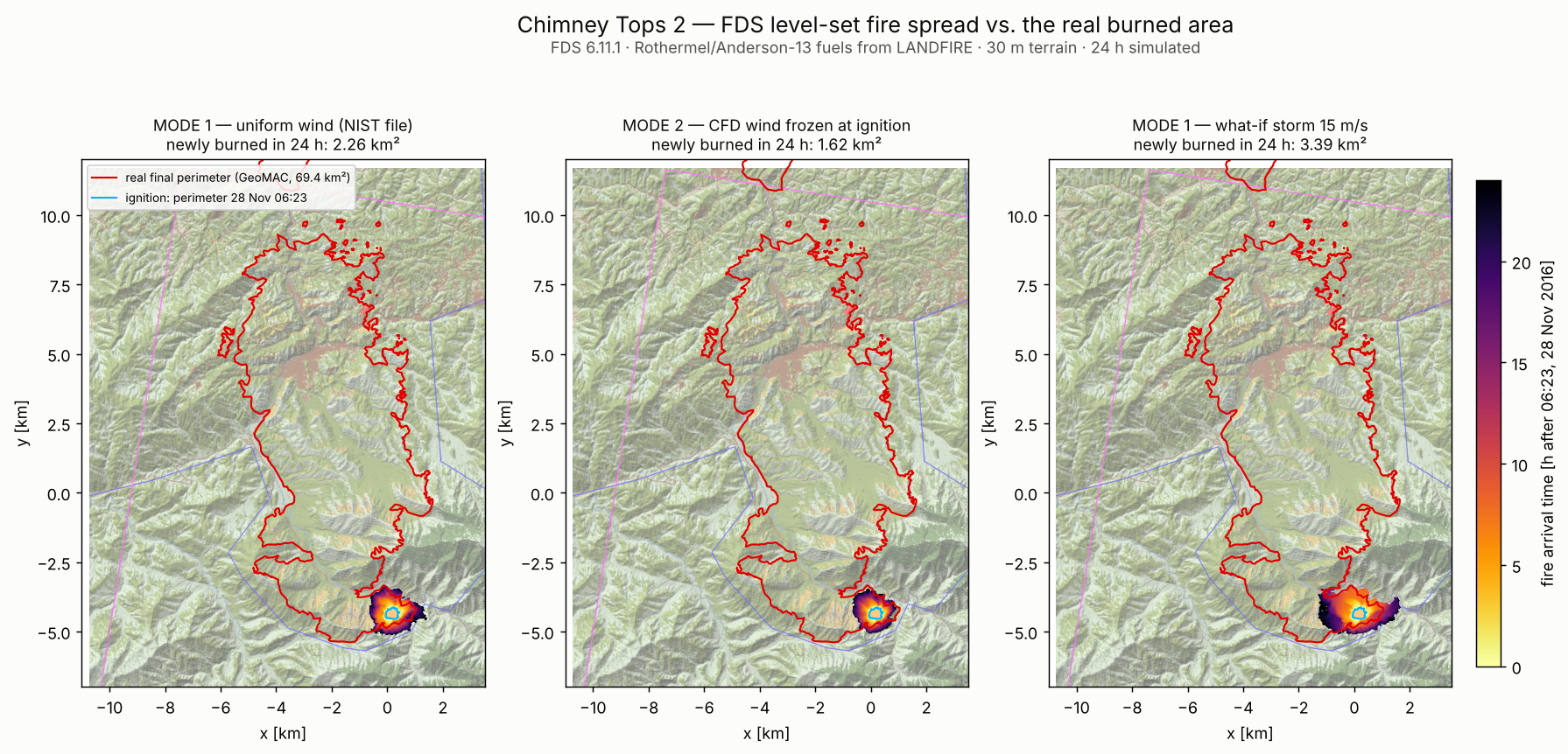
• Mode 2 (wind over the terrain frozen at ignition) burned 1.62 km², less than mode 1 (2.26 km²), likely because the near-ground wind in the valleys is weaker than the uniform profile and its direction stays frozen.
• Mode 1 with DT=10 s gave exactly the same burned area as the default time step (1.07 s) in one seventh of the solver time (344 s vs 2,471 s); billed €2.76 instead of €8.59, mostly fixed overhead.
• The level set burned 2.3 km² around the initial perimeter in 24 h, against 69.4 km² inside the real final perimeter. Even with a 15 m/s what-if storm it stopped at 3.4 km²: the front cannot cross a river and road corridor that the real fire jumped with embers. FDS’s level set does not model spotting.
• Right tool for the job: modes 1–2 for fast scenario studies on large terrains, mode 3 when the local wind matters, mode 4 for short, local fire–atmosphere interaction studies.

Why this case

Wildland and wildland–urban interface (WUI) fires are a growing part of fire safety engineering, and FDS has been extended for them with a level-set fire-spread model on complex terrain (Vanella et al., 2021). The terrain, land use and fuel models are prepared with qgis2fds, the open source QGIS plugin that exports elevation, LANDFIRE fuel classes and georeferencing to an FDS input.

NIST publishes a ready-made qgis2fds example of the Chimney Tops 2 fire in its firemodels/cad repository. The fire started in Great Smoky Mountains National Park on 23 November 2016 and, after days of slow growth, was pushed by an extreme wind event on the afternoon of 28 November out of the park into Gatlinburg, Tennessee (NPS Chimney Tops 2 Fire Review, 2017). The fire, together with other fires in the area, caused 14 deaths. It is a sobering case, and a good one to explain what each FDS wildfire option can and cannot do.

We did not compare FDS versions here: everything ran on FDS 6.11.1. The question is which level-set mode to use, what it costs and what it misses.

Results at a glance

Run	LEVEL_SET_MODE	Wind seen by the fire	Simulated time	Time step	Solver wall time	Billed cost	Burned after 24 h
M1, DT 10 s	1	uniform, NIST wind file	24 h	10 s (locked)	344 s	€2.76	2.26 km²
M1, default DT	1	uniform, NIST wind file	24 h	1.07 s	2,471 s	€8.59	2.26 km²
M2	2	CFD over terrain, frozen at ignition	10 min spin-up + 24 h	1.07 s	18,020 s	€54.24	1.62 km²
M3	3	CFD over terrain, whole run	300 s	1.07 s	5.73 s/step	€6.36	— (extrapolated: €56 per simulated hour)
M4	4	CFD coupled with the fire	120 s	1.07 s	7.28 s/step	€3.95	— (extrapolated: €72 per simulated hour)
M1 what-if storm	1	uniform, synthetic: 2 m/s, then 15 m/s (8–19 h), then 3 m/s, all from 200°	24 h	10 s (locked)	343 s	€2.58	3.39 km²
Reality	—	—	—	—	—	—	69.4 km² inside the final perimeter (GeoMAC), 64.5 km² of it inside the FDS domain

All runs: 96 vCPU hypercore spot (85 MPI processes on physical cores, AMD EPYC 9B45), €10.56 per hour. Billed cost includes boot, end-of-run detection and result upload. Burned areas are the cells burned by the level set outside the initial 0.14 km² perimeter.

The case setup

• Domain: 21.4 × 23.4 km, terrain from 317 to 2,006 m, imported as a single &GEOM binary file (.bingeom, 1.1 M triangles from a 30 m DEM) with the land-use texture for Smokeview.
• Mesh: 15 × 17 = 255 meshes of 48 × 46 × 66 cells, about 30 m in every direction, 37,160,640 cells. The original file uses MULT_ID; we expanded it to 255 explicit &MESH lines grouped three by three with MPI_PROCESS → 85 MPI processes.
• Fuels: LANDFIRE 13 Anderson fuel models mapped to VEG_LSET_FUEL_INDEX. The domain is dominated by closed timber litter (model 8) and hardwood litter (model 9), about 470 of 550 km² of terrain surface. Urban, water and barren cells do not burn.
• Ignition: the GeoMAC perimeter “CHIMNEY 2” of 28 November 2016 at 06:23 (36 acres, 0.14 km²), which matches the 35 acres seen by the infrared flight of 27 November. So t = 0 is the morning of the wind event.
• Wind: the case comes with an hourly wind file (speed and direction ramps on &WIND, 149 h). In the first 24 h it blows 1.4–2.5 m/s from 217–322°. We could not trace its source, and it does not contain the extreme wind of 28 November: the NPS reported gusts up to 87 mph (39 m/s) at the Cove Mountain weather station, 8 miles north-west of the fire’s origin (Wildfire Today, 2016).
• Reference: the GeoMAC final perimeter “CHIMNEY TOPS 2” (12 December 2016, 17,132 acres, 69.4 km²). Part of it lies outside the FDS domain (north-west), and not everything inside a perimeter actually burns.

The four level-set modes in one paragraph each

FDS solves a level-set equation on the terrain surface: the fire front moves with the Rothermel rate of spread computed from fuel, slope and wind at mid-flame height (Rothermel, 1972; Anderson, 1982). The four modes change only where the wind comes from and whether the fire feeds back on it (FDS User’s Guide).

• Mode 1: the flow is not solved (FREEZE_VELOCITY and solid phase only). The fire uses the &WIND profile directly, uniform in space, with its time ramps. Terrain affects spread only through the slope.
• Mode 2: the CFD solves the wind over the terrain until ignition, then the field is frozen and the run continues like mode 1. The wind feels the ridges and valleys, but it stops changing.
• Mode 3: the CFD solves the wind for the whole run, but the fire does not release heat into the gas. The terrain-modified wind follows the time ramps.
• Mode 4: full coupling. The burning cells release heat and smoke, the plume changes the wind, the wind changes the spread rate.

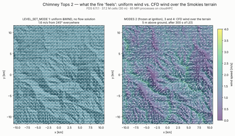
Left: the wind every cell sees in mode 1. Right: the LES wind 5 m above the ground after 300 s of mode 3: 0.4–1.9 m/s (5th–95th percentile), up to 4.8 m/s, channelled by the valleys.

Results

Mode 1: the 10 s trick

In mode 1 nothing limits the time step: with the velocity frozen FDS keeps the initial 1.07 s for the whole run (80,636 steps for 24 h). The level set front moves a few tens of metres per hour (about one 30 m cell per hour), so we locked the step at 10 s:

&TIME T_END=86400., DT=10., LOCK_TIME_STEP=.TRUE. /

The burned cells are identical at 4, 12 and 24 h (intersection over union = 1.000), and the solver time drops from 2,471 s to 344 s. Each step costs about the same (0.03–0.04 s for 37 M cells), so fewer steps means a cheaper run: €2.76 instead of €8.59, most of which is now fixed overhead.

Mode 1 vs. reality

With the NIST wind file the level set burns 2.26 km² in 24 h around the initial 0.14 km² perimeter, spreading about 1–1.3 km from the ignition. Reality: 69.4 km² inside the final perimeter, most of it burned in the night between 28 and 29 November.

The gap is not a bug, and it tells two things:

1. Input weather drives the result. The wind file is weak (≤ 2.5 m/s). To test it we ran a what-if mode 1 case with a synthetic wind, clearly not measured data: all from 200°, 2 m/s until 12:23, ramping to 15 m/s by 14:23, 15 m/s until 01:23, then 3 m/s. The burned area grows by 50 %, to 3.39 km².
2. The level set does not model spotting. In the what-if run the front stops about 1 km north of the ignition on a corridor of water and urban (road) cells in the valley floor. Rothermel spread needs fuel in the next cell. The real fire crossed that corridor, and much more, with embers carried by the wind: spot fires were reported 5 miles from the main fire on the afternoon of 28 November (National Parks Traveler, 2017), and other fires were started by downed power lines.

Mode 2

Mode 2 spent the first 560 steps (10 simulated minutes before the ignition, about 53 min of solver time) solving the LES wind over the terrain at 5.7 s per step, then froze it. After the freeze the run continued for 80,636 steps at 0.18 s per step (€1.81 per simulated hour): much cheaper than the CFD, but about six times slower than mode 1 on the same mesh, and the time step stays at 1.07 s. Total solver time: 5.0 h, billed €54.24.

The result is the opposite of what many expect: the terrain-resolved wind burns less, 1.62 km² after 24 h instead of 2.26 km². Two likely reasons. Near the ground, in the valleys and on the lee slopes, the LES wind is weaker than the uniform &WIND profile (in the mode 3 field after 300 s, 83 % of the cells 5 m above ground are below 1.6 m/s, median 1.24 m/s). And the field is frozen at its ignition-time direction (245°) for the whole day, while mode 1 follows the hourly changes of speed (1.4–2.5 m/s) and direction in the wind file.

If you need mode 2 for a long run, stop it after the spin-up and restart it with DT=10. and LOCK_TIME_STEP=.TRUE.: the frozen field does not care about the step.

Modes 3 and 4: what the CFD costs

Mode 3 ran 300 s and mode 4 ran 120 s: enough to measure the cost per step, not to see the fire move.

• Mode 3: 5.73 s per step, 70 % of it in the pressure solver. One simulated hour (3,360 steps) needs 5.4 h of solver time, about €56. The 24 h of this post would cost about €1,350; the 149 h of the wind file about €8,400.
• Mode 4: 7.28 s per step (the pressure solver as in mode 3, plus radiation and vegetation/geometry work). The heat release stays at about 220 kW from 20 s to 106 s, then jumps to 80 MW at 120 s. One simulated hour: 6.8 h, about €72 at the 1.07 s time step, which held up to 120 s; with a larger fire the step may shrink and the cost grow.

What we learned

• Pick the mode by the question. Scenario studies over large terrains (many wind directions and speeds, ignition points, fuel moistures) belong to modes 1–2: a full day costs a few euros. Mode 3 makes sense when the local wind field drives the answer and the duration is short. Mode 4 is for local studies of fire–atmosphere interaction (plume, smoke, radiation to a building), on a smaller domain and finer grid.
• In mode 1 set DT yourself. Same result, one seventh of the solver time.
• The weather file matters more than the mode. A 6-day wind file without the event’s gusts cannot reproduce the event, whatever the CFD.
• Know what the model leaves out. Rothermel spread with no spotting stops at a road or a stream. Chimney Tops 2 was an ember-driven fire in an extreme mountain-wave wind: the level set gives a lower bound of the spread, not a forecast.
• 37 M cells need memory. Peak memory was 286–312 GiB of the 354 GiB available on 96 hypercore vCPU (81–88 %, about 8–9 kB per cell; the highest with mode 4). Plan the instance on RAM, not only on cores.

Run times and costs

Run	Purpose	Steps	Solver wall time	Billed
M1 sizing (1 h)	time per step	3,360	135 s	€2.25
M2 sizing (10 min spin-up + 30 min)	spin-up cost	—	—	€12.01
M3 (300 s)	cost per step, wind field	280	1,605 s	€6.36
M4 sizing (1 s)	first step	1	12 s	€1.77
M1, DT 10 s (24 h)	result	8,640	344 s	€2.76
M1, default DT (24 h)	check of the 10 s step	80,636	2,471 s	€8.59
M1 what-if storm (24 h)	sensitivity to wind	8,640	343 s	€2.58
M2 (24 h)	result	81,196	18,020 s	€54.24
M4 (120 s)	cost per step with fire	112	815 s	€3.95
Total				€94.51

How to run this case on cloudHPC

1. Download Chimney_Tops_2.fds and Chimney_Tops_2_terrain.bingeom from firemodels/cad. The .png texture is only for Smokeview and is removed by cloudHPC on a new run (only .dat .bdf .txt .py .sh and geometry files like .bingeom are kept).
2. Expand the MULT_ID meshes into explicit &MESH lines: cloudHPC starts one MPI process per &MESH line and a MULT counts as one. Group them with MPI_PROCESS (three per process → 85 processes). The script we used is in the case files.
3. Choose LEVEL_SET_MODE. For mode 2 start at T_BEGIN=-600. so the wind has time to develop before the ignition at t = 0.
4. Mode 1: add DT=10., LOCK_TIME_STEP=.TRUE. to &TIME.
5. Set DT_SLCF (we used 600 s for the 24 h runs): the default 1,000 frames of the original slices produce several GB.
6. Launch on 96 vCPU hypercore spot with fds6.11.1: 85 processes on physical cores and enough RAM for 37 M cells. Add DT_RESTART on &DUMP for long runs; spot is fine, the platform resumes from the last restart.

FAQ

Can FDS simulate wildfires?
Yes. FDS includes a level-set fire-spread model on complex terrain (Rothermel rate of spread with the Anderson fuel models) and a particle-based vegetation model for detailed fire–fuel interaction. Terrain and fuels can be prepared with qgis2fds.

What is LEVEL_SET_MODE in FDS?
It sets how the level-set fire spread is coupled with the wind: 1 = uniform wind, no flow solution; 2 = CFD wind over the terrain frozen at ignition; 3 = CFD wind for the whole run, no heat release; 4 = fully coupled fire and atmosphere.

How expensive is a wildfire simulation in FDS?
For this 37 M cell, 21 × 23 km case on 96 vCPU: about €0.04 per simulated hour in mode 1 with a 10 s time step, €56 in mode 3 and €72 or more in mode 4.

Does the FDS level set model ember spotting?
No. The front advances cell by cell with the Rothermel rate of spread; non-burnable cells such as roads, rivers or urban areas stop it. Ember-driven spread, as in Chimney Tops 2, is not captured.

How do I import real terrain into FDS?
With qgis2fds: in QGIS you choose the extent, DEM, land-use layer and fuel mapping, and the plugin writes the .fds file and a binary &GEOM terrain (.bingeom) with the land use on each face.

References

• Vanella M., McGrattan K., McDermott R., Forney G., Mell W., Gissi E., Fiorucci P. (2021). A Multi-Fidelity Framework for Wildland Fire Behavior Simulations over Complex Terrain. Atmosphere 12(2), 273. doi:10.3390/atmos12020273
• McGrattan K. et al. Fire Dynamics Simulator User’s Guide, NIST Special Publication 1019, FDS 6.11.1. pages.nist.gov/fds-smv
• Rothermel R.C. (1972). A Mathematical Model for Predicting Fire Spread in Wildland Fuels. USDA Forest Service Research Paper INT-115. treesearch 32533
• Anderson H.E. (1982). Aids to Determining Fuel Models for Estimating Fire Behavior. USDA Forest Service GTR INT-122. treesearch 6447
• Wildfire Today (2016). Chimney Tops 2 Fire: NPS statement and weather data. wildfiretoday.com
• National Parks Traveler (2017). Report: Great Smoky Mountains National Park staff not negligent battling deadly Chimney Tops 2 Fire. nationalparkstraveler.org
• National Park Service (2017). Chimney Tops 2 Fire Review — Individual Fire Review Report. npshistory.com
• NIST firemodels/cad, Chimney_Tops_2 case study (qgis2fds 1.0.2 export). github.com/firemodels/cad
• qgis2fds — QGIS plugin to export terrain and land use to FDS. github.com/firetools/qgis2fds
• GeoMAC Historic Fire Perimeters 2000–2018 (perimeters “CHIMNEY 2”, 28/11/2016, and “CHIMNEY TOPS 2”, 12/12/2016), distributed with the case QGIS project.
• LANDFIRE LF 2022 Anderson 13 Fire Behavior Fuel Models (F13) and LF 2020 elevation. landfire.gov

---

CloudHPC is a HPC provider to run engineering simulations on the cloud. CloudHPC provides from 1 to 224 vCPUs for each process in several configuration of HPC infrastructure - both multi-thread and multi-core. Current software ranges includes several CAE, CFD, FEA, FEM software among which OpenFOAM, FDS, Blender and several others.

New users benefit of a FREE trial of 300 vCPU/Hours to be used on the platform in order to test the platform, all each features and verify if it is suitable for their needs

---

Contact Name/Surname *

Company Name *

Company address *

City *

State/Province *

Country *CountryArubaAfghanistanAngolaAnguillaÅland IslandsAlbaniaAndorraUnited Arab EmiratesArgentinaArmeniaAmerican SamoaAntarcticaFrench Southern TerritoriesAntigua and BarbudaAustraliaAustriaAzerbaijanBurundiBelgiumBeninBonaire, Sint Eustatius and SabaBurkina FasoBangladeshBulgariaBahrainBahamasBosnia and HerzegovinaSaint BarthélemyBelarusBelizeBermudaBolivia, Plurinational State ofBrazilBarbadosBrunei DarussalamBhutanBouvet IslandBotswanaCentral African RepublicCanadaCocos (Keeling) IslandsSwitzerlandChileChinaCôte d'IvoireCameroonCongo, The Democratic Republic of theCongoCook IslandsColombiaComorosCabo VerdeCosta RicaCubaCuraçaoChristmas IslandCayman IslandsCyprusCzechiaGermanyDjiboutiDominicaDenmarkDominican RepublicAlgeriaEcuadorEgyptEritreaWestern SaharaSpainEstoniaEthiopiaFinlandFijiFalkland Islands (Malvinas)FranceFaroe IslandsMicronesia, Federated States ofGabonUnited KingdomGeorgiaGuernseyGhanaGibraltarGuineaGuadeloupeGambiaGuinea-BissauEquatorial GuineaGreeceGrenadaGreenlandGuatemalaFrench GuianaGuamGuyanaHong KongHeard Island and McDonald IslandsHondurasCroatiaHaitiHungaryIndonesiaIsle of ManIndiaBritish Indian Ocean TerritoryIrelandIran, Islamic Republic ofIraqIcelandIsraelItalyJamaicaJerseyJordanJapanKazakhstanKenyaKyrgyzstanCambodiaKiribatiSaint Kitts and NevisKorea, Republic ofKuwaitLao People's Democratic RepublicLebanonLiberiaLibyaSaint LuciaLiechtensteinSri LankaLesothoLithuaniaLuxembourgLatviaMacaoSaint Martin (French part)MoroccoMonacoMoldova, Republic ofMadagascarMaldivesMexicoMarshall IslandsNorth MacedoniaMaliMaltaMyanmarMontenegroMongoliaNorthern Mariana IslandsMozambiqueMauritaniaMontserratMartiniqueMauritiusMalawiMalaysiaMayotteNamibiaNew CaledoniaNigerNorfolk IslandNigeriaNicaraguaNiueNetherlandsNorwayNepalNauruNew ZealandOmanPakistanPanamaPitcairnPeruPhilippinesPalauPapua New GuineaPolandPuerto RicoKorea, Democratic People's Republic ofPortugalParaguayPalestine, State ofFrench PolynesiaQatarRéunionRomaniaRussian FederationRwandaSaudi ArabiaSudanSenegalSingaporeSouth Georgia and the South Sandwich IslandsSaint Helena, Ascension and Tristan da CunhaSvalbard and Jan MayenSolomon IslandsSierra LeoneEl SalvadorSan MarinoSomaliaSaint Pierre and MiquelonSerbiaSouth SudanSao Tome and PrincipeSurinameSlovakiaSloveniaSwedenEswatiniSint Maarten (Dutch part)SeychellesSyrian Arab RepublicTurks and Caicos IslandsChadTogoThailandTajikistanTokelauTurkmenistanTimor-LesteTongaTrinidad and TobagoTunisiaTürkiyeTuvaluTaiwan, Province of ChinaTanzania, United Republic ofUgandaUkraineUnited States Minor Outlying IslandsUruguayUnited StatesUzbekistanHoly See (Vatican City State)Saint Vincent and the GrenadinesVenezuela, Bolivarian Republic ofVirgin Islands, BritishVirgin Islands, U.S.Viet NamVanuatuWallis and FutunaSamoaYemenSouth AfricaZambiaZimbabwe

Contact City Email

Email *

Email

Confirm Email

Privacy *

• I accept the privacy conditions

Privacy Policy

Send registration