FDS preCICE adapter: coupling a fire simulation to a structural solver (open source)

TL;DR

• We wrote and released an open-source FDS preCICE adapter (CFD-FEA-SERVICE/fds-precice-adapter, GPL-3.0). It couples FDS 6.11.1 to any solver in the preCICE ecosystem through preCICE 3.3.1.
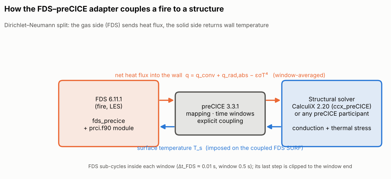
• FDS sends the net heat flux into a wall and gets the wall temperature back from the solid solver, every 0.5 s coupling window. The adapter is one Fortran module plus about 35 changed lines in FDS (a 145-line diff).
• Case 1 (validation): a steel ceiling plate solved through the adapter by an external 1-D conduction solver vs. FDS’s own solid model. After 120 s the temperature rise differs by −3.3 % at the plate centre and 0.0 % at the edge.
• Case 2 (thermo-mechanics): FDS + CalculiX 2.20 on a 5 mm steel plate clamped at both ends under a 300 kW fire. CalculiX’s mid-span axial stress is −176.3 MPa vs. −173.2 MPa from the hand check −E·α·mean(ΔT), a +1.8 % difference. The clamped corners reach about −420 MPa.
• Current limits: explicit coupling only, rectilinear FDS geometry, linear elastic steel in the demo. A cloudHPC app (FDS + preCICE + CalculiX) is on the way.

Why couple FDS to a structural solver?

FDS is the most used fire model in performance-based fire engineering. Its solid-phase heat transfer is mostly one-dimensional through each wall cell (a 3-D option exists for simple obstructions). It has no mechanics at all. When the question becomes “how hot does this beam get, and what does the restraint do to it?”, engineers usually run FDS, export a thermal exposure, and feed it to a finite element (FE) model in a separate, one-way step.

That one-way route is well established:

• NIST described an FDS–FEM method for coupled thermal–structural response (Zhang, SiF’16).
• VTT built FDS2FEM for FDS → Abaqus (Paajanen et al., 2013).
• Liège developed an FDS → SAFIR interface based on transfer files (Tondini, Vassart & Franssen, 2012).

The gap is a two-way, open-source, solver-agnostic connection. In such a connection the structure’s surface temperature feeds back into the fire (re-radiation, convection), and the structural code is a choice rather than a fixed pairing.

preCICE is the open-source coupling library that already does this for OpenFOAM, CalculiX, code_aster, SU2, FEniCSx, OpenRadioss and others (preCICE v2 paper). The adapter overview lists no FDS adapter, so we wrote one.

Results at a glance

Case	What is compared	Reference	FDS–preCICE result	Difference
1 — ceiling plate, centre	Surface temperature rise after 120 s	14.76 K (FDS native 1-D solid)	14.27 K	−3.3 %
1 — ceiling plate, edge	Surface temperature rise after 120 s	8.68 K	8.68 K	0.0 %
1 — ceiling plate, centre	Mean net heat flux 10–120 s	4.37 kW/m²	4.20 kW/m²	−3.9 %
2 — clamped plate, mid-span	Section-mean axial stress σxx at 180 s	−173.2 MPa (−E·α·mean ΔT)	−176.3 MPa (CalculiX)	+1.8 % (max 1.8 % for t ≥ 20 s)
2 — clamped plate	Peak compression (clamped corner) at 180 s	—	−422 MPa	mesh-dependent corner singularity; above yield of S275/S355, elastic result only

How the adapter works

The adapter is a Fortran module (prci.f90) compiled into FDS, plus a small patch (about 35 changed lines) to four FDS source files and the makefile. FDS has no plugin interface, so the result is a separate executable, fds_precice. A standard FDS build is not affected.

• Input: one &PRCI line in the .fds file names the preCICE participant, the config file, the mesh name and the coupled SURF_IDs. A coupled SURF is an ordinary TMP_FRONT surface. That temperature is used until the solid sends its first value.
• Coupling mesh: the centres of all WALL cells on coupled surfaces. Every FDS MPI process registers its own cells, and preCICE handles the parallel partitioning and the mapping to the solid mesh.
• Data sent (Dirichlet–Neumann, default): the net heat flux into the solid, q = q_conv + q_rad,absorbed − εσT_s⁴, in W/m². The usual gas/solid split applies: the low-conductivity side (gas) receives temperature, the high-conductivity side (solid) receives flux.
• Time stepping: FDS sub-cycles inside each preCICE window. Its time step is clipped so it never steps over a window end. The flux sent is the time average over the window, so the structure does not see single LES samples.
• Robin mode: FDS can instead send a sink temperature and an effective heat transfer coefficient (convection plus linearised radiation). It is implemented but not yet tested.
• Not yet supported: implicit coupling (it would need FDS checkpointing), unstructured GEOM surfaces, and FDS restart.

&PRCI PARTICIPANT='Fluid', CONFIG_FILE='../precice-config.xml', MESH_NAME='Fluid-Mesh',
      SURF_ID='PLATE', COUPLING_MODE='DIRICHLET', TEMPERATURE_UNIT='K' /
&SURF ID='PLATE', TMP_FRONT=20., EMISSIVITY=0.9 /
&VENT XB=0.2,1.8,0.8,1.2,2.0,2.0, SURF_ID='PLATE' /

How the runs were set up

Item	Case 1 — ceiling plate	Case 2 — clamped plate
Fire solver	FDS 6.11.1 (tag FDS-6.11.1, GCC 13.3 + Open MPI 4.1.6), 2 meshes, 2 MPI processes, 0.1 m cells (8000)
Coupling	preCICE 3.3.1, serial-explicit, 0.5 s window, nearest-neighbour mapping
Fire	150 kW propane, 0.4 × 0.4 m burner	300 kW propane, 0.4 × 0.4 m burner
Structure	1.0 × 1.0 m steel plate, 10 mm, back insulated	1600 × 400 × 5 mm steel plate, short ends clamped, back adiabatic
Solid solver	Python 1-D implicit conduction per vertex (pyprecice), 0.05 m surface grid	CalculiX 2.20 (preCICE CalculiX adapter 2.20.2), 512 C3D20R, *COUPLED TEMPERATURE-DISPLACEMENT
Steel	ρ 7850 kg/m³, c 460 J/(kg·K), k 45.8 W/(m·K), ε 0.9; case 2 also E 210 GPa, ν 0.3, α 1.2·10⁻⁵ 1/K (constant, linear elastic)
Simulated time	120 s (240 windows)	180 s (360 windows)
Hardware	2-vCPU, 7 GB Linux VM (development machine, not cloudHPC)

Case 1 — ceiling plate: the adapter against FDS’s own solid model

The cleanest check is to solve the same steel twice. In the reference run the plate is an FDS thermally-thick SURF (MATL_ID, BACKING='INSULATED'), solved by FDS’s internal 1-D conduction. In the coupled run the plate is a TMP_FRONT SURF tagged in &PRCI. An external Python participant solves the same 1-D conduction at each point of a 0.05 m surface grid. The fire, mesh and steel properties are identical; only the place where the solid is solved changes.

Point	FDS native	FDS–preCICE	Difference in rise	Max |ΔT| over 10–120 s
Centre (1.0, 1.0)	34.76 °C	34.27 °C	−3.3 %	0.62 K
Edge (0.6, 0.6)	28.68 °C	28.68 °C	0.0 %	0.13 K

What we learned

• The edge point, outside the plume, matches to 0.13 K for the whole run, and its mean flux differs by only +0.2 %: no sign of a systematic bias from the coupling. At the centre, right in the plume, the coupled run is 0.5 K lower after 120 s, in line with the −3.9 % difference in mean heat flux there. The inputs are identical, but the coupling changes the FDS time-step sequence (window-end clipping), so the turbulent plume follows a different history. The centre difference is within what that produces, but a single pair of runs cannot fully separate the two effects; repeated runs would.
• The coupled FDS run took 11.5 % more wall time, and also 11.8 % more time steps. Per step the cost is the same: 25.6 ms vs. 25.7 ms. Exchanging data with preCICE costs nothing measurable at this size. The extra steps come from window-end clipping plus a different time-step history in the two LES runs.
• The flux is window-averaged on purpose. In case 1 a 0.5 s window holds about 40–50 FDS steps (about 58 in case 2), so the solid receives a smooth flux rather than whichever instantaneous LES sample falls at the window end.

Case 2 — thermo-mechanical: FDS fire + CalculiX thermal stress

The second case is the one fire engineers care about. Heat from the fire flows into steel, the steel tries to expand, and the restraint turns that expansion into stress. CalculiX runs a transient *COUPLED TEMPERATURE-DISPLACEMENT analysis with a fixed 0.5 s increment matching the coupling window:

• It reads the FDS heat flux on the face centres of the exposed surface (*DFLUX).
• It writes the nodal temperature of that surface back to FDS.
• Both short ends are fully clamped.

Hand check. If both ends are fixed, the axial force is the same in every cross-section. With constant E and α, its value depends only on the mean temperature rise over the whole plate: σ = −E·α·mean(ΔT). The local formula −E·α·ΔT(mid-span) would overestimate the mid-span compression. The ends stay cooler and give way to the hot centre. Both sides of the check use FE-consistent averages: the volume average of the temperature rise, and the area average of σxx over the mid-span section.

Quantity at t = 180 s	Value
Exposed face temperature, mid-span (CalculiX / as seen by FDS)	137.0 °C / 134.7 °C
Front–back temperature difference, mid-span	0.5 K (max 0.8 K during the run)
Exposed face temperature range	56.4–137.2 °C
Mean temperature rise over the plate (volume average)	68.7 K
Hand check −E·α·mean(ΔT)	−173.2 MPa
CalculiX section-mean σxx at mid-span (area average)	−176.3 MPa (+1.8 %)
Local −E·α·ΔT(mid-span, through-thickness mean) (not applicable, shown for comparison)	−294.2 MPa
Peak compression σxx (clamped corners, mesh-dependent)	−422.0 MPa
Maximum von Mises stress	455.8 MPa
Mid-span deflection	−0.06 mm (|max| 0.12 mm)

What we learned

• The flux sign convention of the FDS adapter (positive into the solid) matches CalculiX’s *DFLUX with no conversion. The CalculiX–FDS temperature pair is consistent: FDS reports 134.7 °C, against 137.0 °C at the nearest CalculiX node. FDS samples a 0.1 m cell and lags by one 0.5 s window.
• The restraint stress follows the hand check within 1.8 % for the whole run after the first 20 s. The bar formula assumes uniaxial stress, but the clamps also block the plate’s expansion across its width at the ends. That is a likely reason why CalculiX is slightly more compressive.
• The corners reach about −420 MPa compression and 456 MPa von Mises, while the hottest point of the plate is only 137 °C and the corners themselves are at about 57 °C. Fully clamped corners are a stress singularity, so these peaks grow with mesh refinement. Even so, the stress level sits above the yield strength of common structural steels, and that is the point of the demo: with a restraint, a modest temperature rise already matters. Treat the numbers as elastic. A design-level result needs temperature-dependent, elastic–plastic steel per EN 1993-1-2. That is the next step.
• The plate barely bends (0.06 mm). Five millimetres of steel equalises the temperature through its thickness within seconds (front–back difference 0.5 K), and the clamps hold it in plane. A thicker section or one-sided insulation would add a thermal gradient and therefore bending.

What is not there yet

We prefer to say this plainly:

• Explicit coupling only. A fire hardly feels the structure on a 0.5 s window, so this is adequate for fire–structure problems. Strongly coupled problems would need implicit coupling, which needs FDS checkpointing.
• Rectilinear geometry only. Coupled surfaces must be OBST or VENT faces; GEOM/CFACE surfaces are not supported yet.
• No FDS restart in a coupled run.
• Robin mode is implemented but untested.
• CalculiX 2.20. The official preCICE CalculiX adapter targets CalculiX 2.20, while cloudHPC currently offers CalculiX up to 2.21 for standalone runs.
• Not run on cloudHPC yet. Both cases ran on a 2-vCPU development machine.

Run times

Run	Simulated time	Wall time	FDS steps	FDS cost per step
Case 1, FDS native (reference)	120 s	259 s	10,093	25.7 ms
Case 1, FDS–preCICE + Python solid	120 s	289 s	11,289	25.6 ms
Case 2, FDS–preCICE + CalculiX	180 s	17.7 min (both participants)	20,861	50.8 ms

All runs used the same 2-vCPU machine, with the solid solver sharing those two cores with the two FDS processes. In case 2, CalculiX solving 512 quadratic elements every window was the slower participant: FDS waited for it, and that is why its cost per step doubled. On cloudHPC each participant will get its own cores. We will add cloudHPC timings and costs when the app is released.

How to run it

Today, on your own Linux machine:

git clone https://github.com/CFD-FEA-SERVICE/fds-precice-adapter
cd fds-precice-adapter
./build.sh                      # clones FDS-6.11.1, applies the patch, builds bin/fds_precice
cd tutorials/clamped-plate-calculix
FDS_PRECICE=../../bin/fds_precice ./run.sh   # needs ccx_preCICE (calculix-precice3 package)
python3 post.py

You need gfortran, Open MPI, preCICE 3.x (libprecice3 package) and, for case 2, the calculix-precice3 package from the preCICE CalculiX adapter releases.

On cloudHPC (coming soon): a coupled app will bundle fds_precice, preCICE 3.3.1 and CalculiX with the preCICE adapter. Lay out the case as in the tutorials: precice-config.xml at the root, a fluid/ folder for FDS and a solid/ folder for CalculiX. Practical tips for both setups:

• FDS meshes: use one &MESH per MPI process and avoid MULT_ID meshes.
• Time stepping: set the CalculiX increment equal to the coupling window (*... , DIRECT) and make the preCICE max-time equal to T_END.
• Interfaces: CalculiX reads Heat-Flux on a faces mesh (a *SURFACE) and writes Temperature on a nodes mesh (an *NSET). That gives two CalculiX interfaces for one physical surface.

FAQ

Can FDS be coupled with a finite element solver?

Yes. Until now this was mostly one-way: you export the FDS thermal exposure (for example the adiabatic surface temperature) and run the FE model afterwards, with tools such as FDS2FEM or FDS–SAFIR interfaces. The FDS preCICE adapter couples FDS at run time and in both directions for heat transfer. It works with any preCICE-enabled code, for example CalculiX or code_aster.

Is the coupling two-way?

Thermally, yes: FDS sends heat flux and receives the structure’s surface temperature, which then drives FDS’s convection and re-radiation. Mechanically, no: structural deformation does not move FDS obstructions. For most fire–structure problems the deformation is too small to change the fire.

Which FDS and preCICE versions does it support?

FDS 6.11.1 and preCICE 3.x (tested with 3.3.1). The adapter is a patch, so each new FDS release needs a rebuild and possibly a small update of the patch.

How is this different from using FDS’s own HT3D solid heat transfer?

FDS’s solid heat transfer is a thermal model only: there is no stress or deformation. With preCICE the solid side can be a full FE code with real geometry, contact, temperature-dependent materials, plasticity and code checks. FDS stays in charge of the fire.

Can I run FDS–CalculiX coupled simulations on cloudHPC?

The coupled app is being prepared; until then you can build and run the open-source adapter yourself. cloudHPC already runs FDS from 6.7.0 to the latest release, CalculiX and preCICE as separate apps.

References

1. Chourdakis, G., Davis, K., Rodenberg, B., Schulte, M., Simonis, F., Uekermann, B. et al. (2022). preCICE v2: A sustainable and user-friendly coupling library. Open Research Europe 2:51. doi:10.12688/openreseurope.14445.2
2. Uekermann, B., Bungartz, H.-J., Cheung Yau, L., Chourdakis, G., Rusch, A. (2017). Official preCICE adapters for standard open-source solvers. 7th GACM Colloquium on Computational Mechanics, Stuttgart. Extended abstract
3. McGrattan, K., McDermott, R., Weinschenk, C., Overholt, K., Hostikka, S., Floyd, J. (2013). Fire Dynamics Simulator Technical Reference Guide, Volume 1: Mathematical Model. NIST SP 1018e6. doi:10.6028/NIST.SP.1018e6
4. Paajanen, A., Korhonen, T., Sippola, M., Hostikka, S., Malendowski, M., Gutkin, R. (2013). FDS2FEM – A tool for coupling fire and structural analyses. IABSE Workshop: Safety, Failures and Robustness of Large Structures, Helsinki, pp. 218–224. doi:10.2749/222137813807054629
5. Tondini, N., Vassart, O., Franssen, J.-M. (2012). Development of an interface between CFD and FE software. Proc. 7th Int. Conf. on Structures in Fire, Zürich, pp. 459–468. doi:10.3929/ethz-a-007050197
6. Zhang, C. (2016). FDS-FEM simulation method and its application to model localized fire tests on steel members. 9th Int. Conf. on Structures in Fire (SiF’16), Princeton. NIST
7. EN 1993-1-2: Eurocode 3 — Design of steel structures — Part 1-2: General rules — Structural fire design.
8. preCICE adapter overview: precice.org/adapters-overview · preCICE CalculiX adapter: github.com/precice/calculix-adapter · FDS source: github.com/firemodels/fds
9. FDS preCICE adapter, inputs and post-processing of this post: github.com/CFD-FEA-SERVICE/fds-precice-adapter

---

CloudHPC is a HPC provider to run engineering simulations on the cloud. CloudHPC provides from 1 to 224 vCPUs for each process in several configuration of HPC infrastructure - both multi-thread and multi-core. Current software ranges includes several CAE, CFD, FEA, FEM software among which OpenFOAM, FDS, Blender and several others.

New users benefit of a FREE trial of 300 vCPU/Hours to be used on the platform in order to test the platform, all each features and verify if it is suitable for their needs

---

Contact Name/Surname *

Company Name *

Company address *

City *

State/Province *

Country *CountryArubaAfghanistanAngolaAnguillaÅland IslandsAlbaniaAndorraUnited Arab EmiratesArgentinaArmeniaAmerican SamoaAntarcticaFrench Southern TerritoriesAntigua and BarbudaAustraliaAustriaAzerbaijanBurundiBelgiumBeninBonaire, Sint Eustatius and SabaBurkina FasoBangladeshBulgariaBahrainBahamasBosnia and HerzegovinaSaint BarthélemyBelarusBelizeBermudaBolivia, Plurinational State ofBrazilBarbadosBrunei DarussalamBhutanBouvet IslandBotswanaCentral African RepublicCanadaCocos (Keeling) IslandsSwitzerlandChileChinaCôte d'IvoireCameroonCongo, The Democratic Republic of theCongoCook IslandsColombiaComorosCabo VerdeCosta RicaCubaCuraçaoChristmas IslandCayman IslandsCyprusCzechiaGermanyDjiboutiDominicaDenmarkDominican RepublicAlgeriaEcuadorEgyptEritreaWestern SaharaSpainEstoniaEthiopiaFinlandFijiFalkland Islands (Malvinas)FranceFaroe IslandsMicronesia, Federated States ofGabonUnited KingdomGeorgiaGuernseyGhanaGibraltarGuineaGuadeloupeGambiaGuinea-BissauEquatorial GuineaGreeceGrenadaGreenlandGuatemalaFrench GuianaGuamGuyanaHong KongHeard Island and McDonald IslandsHondurasCroatiaHaitiHungaryIndonesiaIsle of ManIndiaBritish Indian Ocean TerritoryIrelandIran, Islamic Republic ofIraqIcelandIsraelItalyJamaicaJerseyJordanJapanKazakhstanKenyaKyrgyzstanCambodiaKiribatiSaint Kitts and NevisKorea, Republic ofKuwaitLao People's Democratic RepublicLebanonLiberiaLibyaSaint LuciaLiechtensteinSri LankaLesothoLithuaniaLuxembourgLatviaMacaoSaint Martin (French part)MoroccoMonacoMoldova, Republic ofMadagascarMaldivesMexicoMarshall IslandsNorth MacedoniaMaliMaltaMyanmarMontenegroMongoliaNorthern Mariana IslandsMozambiqueMauritaniaMontserratMartiniqueMauritiusMalawiMalaysiaMayotteNamibiaNew CaledoniaNigerNorfolk IslandNigeriaNicaraguaNiueNetherlandsNorwayNepalNauruNew ZealandOmanPakistanPanamaPitcairnPeruPhilippinesPalauPapua New GuineaPolandPuerto RicoKorea, Democratic People's Republic ofPortugalParaguayPalestine, State ofFrench PolynesiaQatarRéunionRomaniaRussian FederationRwandaSaudi ArabiaSudanSenegalSingaporeSouth Georgia and the South Sandwich IslandsSaint Helena, Ascension and Tristan da CunhaSvalbard and Jan MayenSolomon IslandsSierra LeoneEl SalvadorSan MarinoSomaliaSaint Pierre and MiquelonSerbiaSouth SudanSao Tome and PrincipeSurinameSlovakiaSloveniaSwedenEswatiniSint Maarten (Dutch part)SeychellesSyrian Arab RepublicTurks and Caicos IslandsChadTogoThailandTajikistanTokelauTurkmenistanTimor-LesteTongaTrinidad and TobagoTunisiaTürkiyeTuvaluTaiwan, Province of ChinaTanzania, United Republic ofUgandaUkraineUnited States Minor Outlying IslandsUruguayUnited StatesUzbekistanHoly See (Vatican City State)Saint Vincent and the GrenadinesVenezuela, Bolivarian Republic ofVirgin Islands, BritishVirgin Islands, U.S.Viet NamVanuatuWallis and FutunaSamoaYemenSouth AfricaZambiaZimbabwe

address Contact Name/Surname

Email *

Email

Confirm Email

Privacy *

• I accept the privacy conditions

Privacy Policy

Send registration