LIGGGHTS vs LAMMPS for DEM: validation and scaling on cloudHPC

Why compare LIGGGHTS and LAMMPS now?

LIGGGHTS (“LAMMPS Improved for General Granular and Granular Heat Transfer Simulations”) was forked from a 2012 version of LAMMPS and became the open-source reference for the Discrete Element Method (DEM). Its public branch has been frozen at 3.8.0 since 30 November 2017 (version history). Meanwhile LAMMPS itself kept moving: its pair_style granular now offers Hertz, JKR and DMT normal models, Mindlin tangential contacts, rolling and twisting resistance, all in the parent code that is actively maintained.

So the practical question for anyone starting a DEM project today is simple: is the specialised fork still worth using, or has the parent caught up? Both codes are available on cloudHPC, so we set up identical cases and let the numbers answer.

Results at a glance

Case	Metric	Reference	LIGGGHTS	LAMMPS
1. Hertz impact	contact time, 0.1–10 m/s	Hertz (analytical)	max error 0.013 %	max error 0.014 %
1. Hertz impact	restitution, input e = 0.3	0.30	0.300	0.440 (tsuji, 7 Feb 2024 build)
2. Silo discharge	flow rate W, D0 = 24 mm	Beverloo, C = 0.58	0.2049 kg/s	0.2034 kg/s
2. Silo discharge	fitted Beverloo C / k	0.58 / 1.5 (textbook)	0.583 / 0.51	0.580 / 0.50
3. Column collapse	runout, a ≈ 3	Lube et al. 2004	+3.5 %	+3.4 %
3. Column collapse	runout, a ≈ 1	Lube et al. 2004	−9.7 %	−9.7 %
Scaling	loop time, 818 k particles, 192 cores	—	69.5 s	86.9 s
Speed	LAMMPS / LIGGGHTS time ratio	—	1	1.15–1.25

How the runs were set up

• Solvers: LIGGGHTS-PUBLIC 3.8.0 (pair_style gran model hertz tangential history) and LAMMPS with the GRANULAR package, the 7 Feb 2024 build available on cloudHPC at the time of testing (pair_style granular hertz/material … tangential mindlin … damping tsuji).
• Same input data: one Python generator writes a single data file per case. LIGGGHTS (atom_style granular) and LAMMPS (atom_style sphere) read the same id type diameter density x y z lines, so both codes start from identical particle positions and diameters.
• Material: soda-lime glass beads, ρ = 2500 kg/m³, E = 10 MPa (softened, as usual in DEM), ν = 0.3, e = 0.9, μ = 0.5, ±5 % size polydispersity.
• Walls: analytic cylinders in both codes. Floors and the silo base are frozen particles (more on why below).
• Machines: cloudHPC hypercore instances (physical cores, one MPI process per core), regular (non-preemptible) instances so that timings are not disturbed.

Case 1 — Hertz impact: contact time and restitution

Nine pairs of 4 mm spheres collide head-on. Five pairs test the restitution (e = 0.3 → 1.0 at 1 m/s), four more test the Hertz contact time over two decades of impact velocity (0.1 → 10 m/s, elastic). The contact time is measured from the overlap history, the restitution from the velocities before and after contact.

Input e	LIGGGHTS measured e	LAMMPS (tsuji) measured e	LAMMPS error
0.3	0.300	0.440	+47 %
0.5	0.500	0.616	+23 %
0.7	0.700	0.778	+11 %
0.9	0.900	0.928	+3 %
1.0	1.000	1.000	0 %

What we learned. The elastic part of the contact law is identical and exact in both codes: contact times match the Hertz solution within 0.014 % from 0.1 to 10 m/s. The damping is not. LIGGGHTS reproduces the requested restitution exactly. The LAMMPS tsuji model in the 7 Feb 2024 build returns a bouncier contact, and the error grows as e decreases.

The LAMMPS documentation explains why: a √2 factor in the Tsuji damping (from Marshall, 2009) was missing in earlier versions and was added in a later release. We checked it with the same LAMMPS build (run locally, inputs and log in the package): feeding it an input that includes the √2 factor brings the measured e back to 0.300 / 0.500 / 0.700 / 0.900. Newer LAMMPS versions also provide damping coeff_restitution, whose formula is the same one LIGGGHTS uses. Not available in the build we tested, so for cases 2 and 3 we used a calibrated tsuji input of 0.862, which gives the target e = 0.9 in LAMMPS.

Practical rule: whatever DEM code you use, run a two-particle impact test before trusting a restitution coefficient. It takes seconds on cloudHPC (our impact run cost €0.01).

Case 2 — Silo discharge vs Beverloo

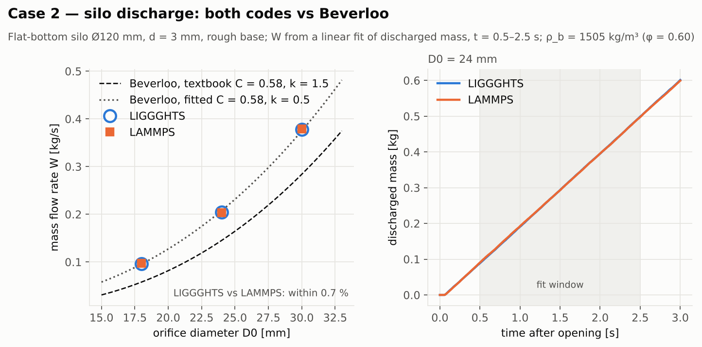
A flat-bottom cylindrical silo (Ø 120 mm) is filled with ~66 600 beads of 3 mm, settled for 0.7 s, then the orifice is opened (D0 = 18, 24, 30 mm). The mass flow rate W comes from a linear fit of discharged mass between 0.5 and 2.5 s. The reference is the Beverloo correlation, W = C ρ_b √g (D0 − k d)^2.5, with ρ_b = 1505 kg/m³ from the measured settled packing (φ = 0.60).

D0 [mm]	W LIGGGHTS [kg/s]	W LAMMPS [kg/s]	Difference	Beverloo textbook [kg/s]
18	0.0967	0.0971	−0.4 %	0.0579
24	0.2049	0.2034	+0.7 %	0.1452
30	0.3783	0.3785	−0.1 %	0.2839

What we learned. The two codes are indistinguishable: within 0.7 % at every orifice, with practically overlapping discharge curves. Both sit 33–68 % above the textbook Beverloo curve, but the fit tells the story: C = 0.583 (LIGGGHTS) and 0.580 (LAMMPS), the textbook 0.58, and k ≈ 0.5 instead of 1.5. The difference is geometric: our orifice rim is made of spheres, so the opening widens by up to one bead diameter just above the base. That shifts the “empty annulus” term by about one d (1.5 − 1 ≈ 0.5).

A modelling note. We first tried to build the perforated base with a LAMMPS region wall (a slab minus a cylinder). Region walls cannot represent the sharp edge of a hole: particles near the rim fell through or were ejected. LIGGGHTS can use an STL mesh plate instead. To keep the geometry identical in both codes we used the classic DEM approach: a rough base of frozen particles with the orifice cut out and a frozen plug that is deleted to open the silo.

Case 3 — Granular column collapse vs experiments

A column of 2 mm beads (initial radius r_i = 30 mm, aspect ratio a = h_i / r_i ≈ 1 and ≈ 3) settles inside a cylinder, which is then removed instantly. The final runout r∞ is compared with the experimental scaling of Lube et al. (2004): r∞ = r_i (1 + 1.24 a) for a < 1.7 and r∞ = r_i (1 + 1.6 a^½) for a > 1.7. Runout is measured as the edge of the continuous deposit (annulus coverage below 50 %), so isolated rolling grains do not inflate it. A third run adds rolling resistance (μ_r = 0.1): rolling_friction cdt in LIGGGHTS, rolling sds in LAMMPS.

Case	a (LIGGGHTS / LAMMPS)	r∞ LIGGGHTS [mm]	r∞ LAMMPS [mm]	Lube et al. [mm] (LIGGGHTS / LAMMPS a)	Error LIGGGHTS / LAMMPS
a ≈ 1	1.04 / 1.04	62	62	68.6 / 68.7	−9.7 % / −9.7 %
a ≈ 3	2.92 / 2.93	116	116	112.0 / 112.2	+3.5 % / +3.4 %
a ≈ 3, μ_r = 0.1	3.02 / 3.01	108	112	113.4 / 113.3	−4.8 % / −1.1 %

What we learned. Without rolling resistance the two codes give the same runout and the same deposit profile. The tall column (a ≈ 3) is within 3.5 % of the experiment; the squat column (a ≈ 1) stops about 10 % short, a known sensitivity of short columns to friction and initial packing. With rolling resistance the codes diverge by two bins (4 mm), because cdt and sds are different models: same μ_r, different torque law. If your application needs rolling resistance (non-spherical grains approximated by spheres), calibrate it in the code you will use.

Speed and scaling (818 k particles)

A dense lattice of 805 500 flowing beads (d = 1 mm) on a 12 684-bead base (818 339 particles including the orifice plug) discharges for 30 000 steps on hypercore instances from 8 to 192 cores. We report the solver loop time from each log (instance boot and result upload excluded).

Cores	LIGGGHTS [s]	LAMMPS [s]	LAMMPS / LIGGGHTS	Efficiency LIGGGHTS / LAMMPS	Solver cost LIGGGHTS / LAMMPS
8	640.8	768.2	1.20	100 % / 100 %	€0.31 / €0.38
16	526.5	646.8	1.23	61 % / 59 %	€0.51 / €0.63
32	339.5	389.3	1.15	47 % / 49 %	€0.66 / €0.76
48	242.2	281.0	1.16	44 % / 46 %	€0.71 / €0.82
96	119.4	149.8	1.25	45 % / 43 %	€0.70 / €0.88
192	69.5	86.9	1.25	38 % / 37 %	€0.82 / €1.02

Solver cost = loop time × cores × €0.22 per vCPU-hour (regular hypercore).

What we learned.

• LIGGGHTS is consistently 15–25 % faster than LAMMPS on the same physics. The same gap appears in the silo (904 s vs 1124 s at D0 = 24 mm) and collapse runs (1067 s vs 1330 s at a ≈ 3).
• Both codes scale the same way: 9.2× (LIGGGHTS) and 8.8× (LAMMPS) from 8 to 192 cores. The modest efficiency is geometry, not the codes. A cylindrical bed in a Cartesian box leaves many subdomains nearly empty (at 192 ranks, 80 of them held fewer than 1 200 of the 818 k particles), and the jump from 8 to 16 ranks puts a whole layer of subdomains below the floor. A balance command or a tighter box would help both codes equally.
• In euros, the fastest solution is not the cheapest: 8 cores cost €0.31 of solver time, 192 cores €0.82, for a 9× shorter wait.

Run times and costs

Series	Runs	Instance	Billed cost
Sizing + impact	3	16 vCPU hypercore / 2 vCPU highcore	€0.78
Silo discharge (3 orifices × 2 codes)	6	16 vCPU hypercore, regular	€13.03
Column collapse (3 cases × 2 codes)	6	16 vCPU hypercore, regular	€13.52
Scaling (6 sizes × 2 codes)	12	8–192 vCPU hypercore, regular	€73.36
Total	27		€100.69

The billed cost includes instance boot, result upload and shutdown, not only the solver. For the 192-core scaling runs the solver ran for about 70–90 s but each instance was billed for about 26–27 minutes. For short benchmark runs the overhead dominates, so run short jobs on few cores and keep large instances for long simulations.

How to run LIGGGHTS and LAMMPS DEM cases on cloudHPC

1. LIGGGHTS: upload a folder with one input file whose name starts with in (e.g. in.hopper) plus meshes and data files referenced with relative paths. Other files must not start with in (rename inlet.stl to plate_inlet.stl).
2. LAMMPS: input files named in.*, *.in, *.lmp or *.lammps. Several main inputs run one after the other; variables must be defined inside the input (no -var on the command line). With one input the log is log.lammps, with several it is log.<input>.lammps.
3. Cores: both codes run one MPI process per physical core. Use hypercore or highcore; on hyperthreaded types only half the selected vCPU are used.
4. Check the restitution in your LAMMPS build with a two-particle test before production (see Case 1).
5. Size the box to the particles, not to the loose fill: empty subdomains made our silo runs about twice as slow as necessary.
6. Download your results: cloudHPC storage is cleaned automatically after 60 days.

FAQ

Is LIGGGHTS still maintained?

The public branch, LIGGGHTS-PUBLIC, has had no release since 3.8.0 (November 2017). It still compiles and runs well, and in our tests it was the faster of the two codes.

Can LAMMPS replace LIGGGHTS for DEM?

For spherical particles with Hertz-Mindlin contacts, yes: in our tests the physics matched within 0.7 % (silo) and to the same 2 mm (collapse, without rolling resistance). Check the damping model in your LAMMPS version and expect runs to be 15–25 % slower than LIGGGHTS.

Why does my LAMMPS granular simulation have the wrong coefficient of restitution?

In LAMMPS versions before the √2 correction, damping tsuji under-damps the contact (e = 0.44 instead of 0.3 in our test). Use damping coeff_restitution in newer versions, or calibrate the tsuji input with a two-particle impact.

How many cores should I use for a DEM simulation?

In our test, parallel efficiency fell below 50 % once each core had fewer than about 25 000 particles (cylindrical geometry, default decomposition). If you pay per core-hour, fewer cores are cheaper; if the deadline matters, 96 cores cut the solver time by about 5× and 192 cores by about 9× compared with 8 cores.

Does LIGGGHTS support STL walls that LAMMPS does not?

Yes. LIGGGHTS can use triangulated STL meshes as walls (fix mesh/surface + fix wall/gran). LAMMPS granular walls are analytic primitives or regions, and region walls do not handle sharp edges such as an orifice rim. For complex equipment geometry this is still a strong reason to choose LIGGGHTS.

References

1. C. Kloss, C. Goniva, A. Hager, S. Amberger, S. Pirker, Models, algorithms and validation for opensource DEM and CFD–DEM, Progress in Computational Fluid Dynamics 12 (2012) 140–152. doi:10.1504/PCFD.2012.047457
2. A. P. Thompson et al., LAMMPS — a flexible simulation tool for particle-based materials modeling at the atomic, meso, and continuum scales, Computer Physics Communications 271 (2022) 108171. doi:10.1016/j.cpc.2021.108171
3. W. A. Beverloo, H. A. Leniger, J. van de Velde, The flow of granular solids through orifices, Chemical Engineering Science 15 (1961) 260–269. doi:10.1016/0009-2509(61)85030-6
4. G. Lube, H. E. Huppert, R. S. J. Sparks, M. A. Hallworth, Axisymmetric collapses of granular columns, Journal of Fluid Mechanics 508 (2004) 175–199. doi:10.1017/S0022112004009036
5. Y. Tsuji, T. Tanaka, T. Ishida, Lagrangian numerical simulation of plug flow of cohesionless particles in a horizontal pipe, Powder Technology 71 (1992) 239–250. doi:10.1016/0032-5910(92)88030-L
6. K. L. Johnson, Contact Mechanics, Cambridge University Press, 1985. doi:10.1017/CBO9781139171731
7. LAMMPS documentation, pair_style granular (damping models, √2 correction of the Tsuji model). docs.lammps.org/pair_granular.html
8. CFDEM®project, LIGGGHTS® version history. cfdem.com/liggghtsr-version-history
9. LIGGGHTS-PUBLIC source repository. github.com/CFDEMproject/LIGGGHTS-PUBLIC

---

CloudHPC is a HPC provider to run engineering simulations on the cloud. CloudHPC provides from 1 to 224 vCPUs for each process in several configuration of HPC infrastructure - both multi-thread and multi-core. Current software ranges includes several CAE, CFD, FEA, FEM software among which OpenFOAM, FDS, Blender and several others.

New users benefit of a FREE trial of 300 vCPU/Hours to be used on the platform in order to test the platform, all each features and verify if it is suitable for their needs

---

Contact Name/Surname *

Company Name *

Company address *

City *

State/Province *

Country *CountryArubaAfghanistanAngolaAnguillaÅland IslandsAlbaniaAndorraUnited Arab EmiratesArgentinaArmeniaAmerican SamoaAntarcticaFrench Southern TerritoriesAntigua and BarbudaAustraliaAustriaAzerbaijanBurundiBelgiumBeninBonaire, Sint Eustatius and SabaBurkina FasoBangladeshBulgariaBahrainBahamasBosnia and HerzegovinaSaint BarthélemyBelarusBelizeBermudaBolivia, Plurinational State ofBrazilBarbadosBrunei DarussalamBhutanBouvet IslandBotswanaCentral African RepublicCanadaCocos (Keeling) IslandsSwitzerlandChileChinaCôte d'IvoireCameroonCongo, The Democratic Republic of theCongoCook IslandsColombiaComorosCabo VerdeCosta RicaCubaCuraçaoChristmas IslandCayman IslandsCyprusCzechiaGermanyDjiboutiDominicaDenmarkDominican RepublicAlgeriaEcuadorEgyptEritreaWestern SaharaSpainEstoniaEthiopiaFinlandFijiFalkland Islands (Malvinas)FranceFaroe IslandsMicronesia, Federated States ofGabonUnited KingdomGeorgiaGuernseyGhanaGibraltarGuineaGuadeloupeGambiaGuinea-BissauEquatorial GuineaGreeceGrenadaGreenlandGuatemalaFrench GuianaGuamGuyanaHong KongHeard Island and McDonald IslandsHondurasCroatiaHaitiHungaryIndonesiaIsle of ManIndiaBritish Indian Ocean TerritoryIrelandIran, Islamic Republic ofIraqIcelandIsraelItalyJamaicaJerseyJordanJapanKazakhstanKenyaKyrgyzstanCambodiaKiribatiSaint Kitts and NevisKorea, Republic ofKuwaitLao People's Democratic RepublicLebanonLiberiaLibyaSaint LuciaLiechtensteinSri LankaLesothoLithuaniaLuxembourgLatviaMacaoSaint Martin (French part)MoroccoMonacoMoldova, Republic ofMadagascarMaldivesMexicoMarshall IslandsNorth MacedoniaMaliMaltaMyanmarMontenegroMongoliaNorthern Mariana IslandsMozambiqueMauritaniaMontserratMartiniqueMauritiusMalawiMalaysiaMayotteNamibiaNew CaledoniaNigerNorfolk IslandNigeriaNicaraguaNiueNetherlandsNorwayNepalNauruNew ZealandOmanPakistanPanamaPitcairnPeruPhilippinesPalauPapua New GuineaPolandPuerto RicoKorea, Democratic People's Republic ofPortugalParaguayPalestine, State ofFrench PolynesiaQatarRéunionRomaniaRussian FederationRwandaSaudi ArabiaSudanSenegalSingaporeSouth Georgia and the South Sandwich IslandsSaint Helena, Ascension and Tristan da CunhaSvalbard and Jan MayenSolomon IslandsSierra LeoneEl SalvadorSan MarinoSomaliaSaint Pierre and MiquelonSerbiaSouth SudanSao Tome and PrincipeSurinameSlovakiaSloveniaSwedenEswatiniSint Maarten (Dutch part)SeychellesSyrian Arab RepublicTurks and Caicos IslandsChadTogoThailandTajikistanTokelauTurkmenistanTimor-LesteTongaTrinidad and TobagoTunisiaTürkiyeTuvaluTaiwan, Province of ChinaTanzania, United Republic ofUgandaUkraineUnited States Minor Outlying IslandsUruguayUnited StatesUzbekistanHoly See (Vatican City State)Saint Vincent and the GrenadinesVenezuela, Bolivarian Republic ofVirgin Islands, BritishVirgin Islands, U.S.Viet NamVanuatuWallis and FutunaSamoaYemenSouth AfricaZambiaZimbabwe

Email *

Email

Confirm Email

Privacy *

• I accept the privacy conditions

Privacy Policy

PageURL State/Province Email

Send registration