OpenFOAM with a GUI: two BARAM tutorials on cloudHPC (pipe flow and Ahmed body)
TL;DR
- BARAM Mesh and BARAM Flow are open-source graphical interfaces that set up snappyHexMesh and an OpenFOAM-based solver without touching a dictionary.
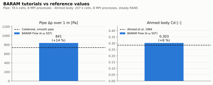
- Tutorial 1, turbulent pipe flow (water, Re ≈ 88,000, 78 k cells): pressure drop 841 Pa vs 740 Pa from Colebrook (+14 %), converged in 239 iterations, under a minute on 8 cores.
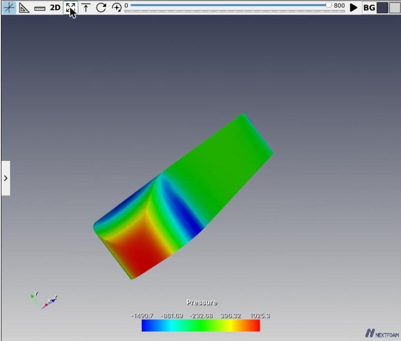
- Tutorial 2, Ahmed body 25° (air, 40 m/s, 207 k cells, half model): Cd = 0.303 vs 0.285 measured by Ahmed et al. (+6 %), about 2 minutes on 8 cores.
- Everything (Salome for the geometry, BARAM Mesh, BARAM Flow) runs in a browser on a cloudHPC remote desktop started with the
ubuntu-staticapp; no local installation. - Salome geometry scripts and every BARAM setting are included in the post.
Why these two tutorials
Every year we run a CFD training for engineering students at the University of Padova. Most of them have never run a simulation, so we want them to see the whole chain (geometry → mesh → solver → results → validation) in one afternoon. Writing OpenFOAM dictionaries by hand is the wrong first step for that audience.
BARAM, developed by NEXTfoam, covers exactly this gap: BARAM Mesh is a step-by-step front-end for snappyHexMesh, BARAM Flow sets up and runs the solver, and both write standard OpenFOAM case files that students can open later. We picked two cases with a known answer, so the class ends with a validation and not just with a nice picture:
- a straight pipe, checked against the Moody diagram (Colebrook equation);
- the Ahmed body, the simplified car used as a reference for automotive aerodynamics since 1984.
Results at a glance
| Case | Cells | Model | Quantity | BARAM | Reference | Difference |
|---|---|---|---|---|---|---|
| Pipe, D 50 mm, L 1 m, 2 m/s water | 78,229 | steady k-ω SST | Δp over 1 m | 841 Pa | 740 Pa (Colebrook, smooth) | +14 % |
| Ahmed body, 25° slant, 40 m/s air | 207,022 | steady k-ω SST | Cd | 0.303 | 0.285 (Ahmed et al. 1984) | +6 % |
How the runs were set up
- Software: Salome for the geometry, BARAM Mesh and BARAM Flow for mesh and solver, all pre-installed on the cloudHPC remote desktop.
- Machine: cloudHPC remote desktop started with the
ubuntu-staticapp, the one that gives a browser-based desktop; both solver runs in parallel on 8 MPI processes (BARAM runs the decomposition for you: Parallel › Environment). - Turbulence: k-ω SST in both cases; pressure-based steady solver (SIMPLE) with the BARAM default schemes and under-relaxation, convergence criteria lowered to 1·10⁻⁵.
Tutorial 1: turbulent flow in a straight pipe
Geometry in Salome
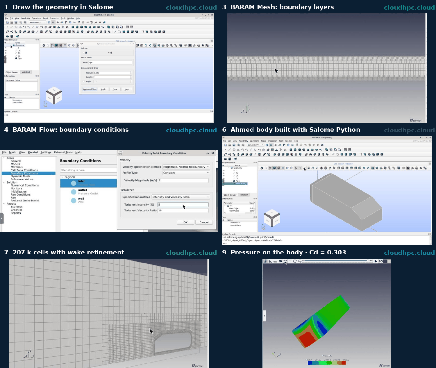
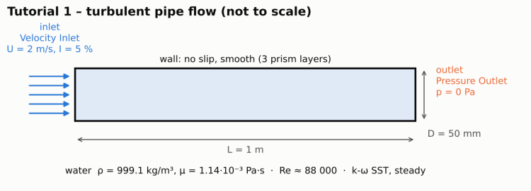
A cylinder of radius 25 mm and length 1 m (Geometry › New Entity › Primitives › Cylinder), exploded into its three faces, each exported as a separate STL: inlet.stl, wall.stl, outlet.stl. One STL per boundary means the OpenFOAM patches are already named when the geometry reaches the mesher. The same steps as a Python script are in the appendix at the end of the post.

Mesh in BARAM Mesh
BARAM Mesh follows the snappyHexMesh steps from left to right: Geometry → Region → Base Grid → Castellation → Snap → Boundary Layer → Export.
| Step | What we set | Why |
|---|---|---|
| Geometry | import the 3 STL files, rename the surfaces | names become the OpenFOAM patches |
| Region | point (0.003, 0.002, 0.7) | must lie inside the fluid and not on a cell face |
| Base grid | 10 × 10 × 200 → 5 mm cubes | keep base cells as close to cubes as possible |
| Castellation | level 1 on all surfaces | 2.5 mm cells near the boundary |
| Snap | defaults | projects the staircase onto the round wall |
| Boundary layer | 3 layers on wall, final layer 0.4, expansion 1.2 |
near-wall resolution |
Result: 78,229 cells, maximum non-orthogonality 30.5°.


Solver in BARAM Flow
Export as BaramFlow project and tick Run BaramFlow on Exported Project. Then:
- Models: turbulence k-ω SST, energy off;
- Materials: add
waterLiquidfrom the database and assign it in Cell Zone Conditions (the default is air, a classic beginner’s mistake); - Boundary Conditions: Velocity Inlet 2 m/s with 5 % intensity, Pressure Outlet 0 Pa, wall no slip;
- Monitors: area-weighted average pressure on the inlet, which is directly the pressure drop of the pipe;
- Initialization: Uz = 2 m/s.

Results
The run converges in 239 iterations. The section at z = 0.9 m shows the flat turbulent profile, with a peak of 2.35 m/s (1.17 × the mean velocity).

The inlet pressure settles at 841 Pa. The Colebrook equation for a smooth pipe at Re = 87,600 gives f = 0.0185 and Δp = 740 Pa: BARAM is 14 % higher.
What we learned. The gap is expected and it is a good classroom discussion:
- with L/D = 20 the flow is not fully developed (entrance length about 30 D for this Re), and the developing region has higher wall friction than the fully developed value used by Colebrook;
- wall y+ is 28–43, so the wall treatment relies on wall functions instead of resolving the viscous sublayer.
The natural exercise is a 3 m pipe, measuring Δp only between z = 2 m and z = 3 m, and a refined boundary layer for y+ ≈ 1.

Tutorial 2: the Ahmed body

Geometry in Salome
The body is 1044 × 389 × 288 mm, with a 100 mm radius on the four front edges, a 25° rear slant and 50 mm ground clearance. A few lines of Salome Python build it (box, fillet on the front edges, cut with a rotated box) and export one STL. Change one number to get the 35° variant. The script is in the appendix.

Mesh in BARAM Mesh
- Wind tunnel: a Hex6 volume from x = −2 m to 6 m, y = 0 to 1.5 m, z = 0 to 1.5 m. It is a half model: the plane y = 0 is a symmetry plane, which halves the cell count.
- Wake box: a second Hex from x = −0.3 to 2 m with its surface type set to None, so it is used only for refinement and does not become a boundary.
- Base grid: Use Hex6 = domain, 80 × 15 × 15 cells (0.1 m).
- Refinement: level 4 on the body surface and feature edges (6.25 mm cells), level 2 in the wake box (25 mm).
- Boundary layer: 5 layers on the body, expansion 1.2.
Result: 207,022 cells.

Solver in BARAM Flow
| Patch | Type | Settings |
|---|---|---|
| domain_xMin | Velocity Inlet | 40 m/s, I = 0.5 % |
| domain_xMax | Pressure Outlet | 0 Pa |
| domain_yMin (y = 0), domain_yMax, domain_zMax | Symmetry | – |
| domain_zMin | Wall | fixed floor |
| body | Wall | no slip |
For the drag coefficient, Reference Values must match the half model: A = 0.056 m² (half of the 0.389 × 0.288 m frontal area), U = 40 m/s, ρ = 1.225 kg/m³. A Force Monitor on body (drag along x, lift along z) plots Cd and Cl during the run.

Results
800 iterations on 8 cores took about 2 minutes. Residuals stall between 10⁻³ and 10⁻⁵ and Cd oscillates between 0.302 and 0.304: the wake of a bluff body is unsteady, so a steady RANS solver never fully settles. On this type of case, judge convergence on the monitored force, not on the residuals.


Cd = 0.303 against 0.285 measured by Ahmed et al.: +6 %, a good number for a 2-minute run on a coarse mesh. To go further:
- a mesh study (level 5 on the body, level 3 in the wake) and a y+ check on the body;
- a transient run or a hybrid RANS-LES, because the 25° slant sits right at the edge of the separation regime, which steady RANS models struggle to predict;
- a moving floor at 40 m/s, as in a real automotive wind tunnel.
Run times
| Case | Cells | Cores | Iterations | Wall time |
|---|---|---|---|---|
| Pipe | 78,229 | 8 | 239 (converged) | under 1 min |
| Ahmed body | 207,022 | 8 | 800 | about 2 min |
Both runs fit comfortably in an interactive remote desktop session; the meshing steps took a few seconds each. Larger meshes (mesh studies, transient runs) are better sent to dedicated compute nodes on cloudHPC.
How to run these tutorials on cloudHPC
- Launch the
ubuntu-staticapp from the cloudHPC dashboard: it starts a browser-based remote desktop with Salome, BARAM Mesh and BARAM Flow already installed. - Paste the scripts of the appendix in the Salome Python console: the STL files land in
~/Desktop/tutorial1_pipeand~/Desktop/tutorial2_ahmed. - Follow the settings in the tables above in BARAM Mesh, export to BARAM Flow, set Parallel › Environment to the number of cores of your desktop and run.
- Remember to stop the remote desktop when you are done: it is billed until it is stopped.
FAQ
Is BARAM free?
Yes. BARAM Mesh and BARAM Flow are open source (GPL-3.0) and developed by NEXTfoam; the source is on GitHub.
Does BARAM generate standard OpenFOAM cases?
Yes. BARAM Mesh writes a snappyHexMesh-based mesh in OpenFOAM format and BARAM Flow writes the usual 0/, constant/ and system/ folders, so you can open and edit the dictionaries later.
Why is the pipe pressure drop 14 % higher than the Moody diagram?
The pipe is only 20 diameters long, so the flow is still developing, and wall y+ is around 30. A longer pipe measured far from the inlet and a finer boundary layer bring the result closer to Colebrook.
Why don’t the residuals drop on the Ahmed body?
The wake behind a bluff body is unsteady. A steady RANS run keeps oscillating, so use the drag coefficient monitor (stable within ±0.001 here) to judge convergence.
How do I get a remote desktop with BARAM on cloudHPC?
Launch the ubuntu-static app: it opens a Linux desktop in the browser with Salome, BARAM Mesh and BARAM Flow pre-installed. Stop it when you finish, because it is billed until stopped.
What reference area should I use for a half model?
Half of the frontal area: 0.056 m² for the Ahmed body, otherwise Cd comes out half of the right value.
Appendix: Salome scripts
Pipe
# Tutorial 1 - straight pipe for BARAM Mesh. Run in the Salome Python console (File > Load Script).
import os, salome, GEOM
from salome.geom import geomBuilder
salome.salome_init()
geompy = geomBuilder.New()
out = os.path.expanduser('~/Desktop/tutorial1_pipe'); os.makedirs(out, exist_ok=True)
pipe = geompy.MakeCylinderRH(0.025, 1.0)          # R = 25 mm, L = 1 m, axis +Z
geompy.addToStudy(pipe, 'Pipe')
faces = geompy.ExtractShapes(pipe, geompy.ShapeType['FACE'], True)
# name faces by the Z of their centre of gravity: 0 -> inlet, 1 -> outlet, 0.5 -> wall
for f in faces:
    z = geompy.PointCoordinates(geompy.MakeCDG(f))[2]
    name = 'inlet' if z < 0.01 else 'outlet' if z > 0.99 else 'wall'
    geompy.ExportSTL(f, f'{out}/{name}.stl', True, 1e-4, False)
print(os.listdir(out))
Ahmed body
# Tutorial 2 - Ahmed body (25 deg slant) for BARAM Mesh. Run in the Salome Python console.
import os, math, salome, GEOM
from salome.geom import geomBuilder
salome.salome_init()
geompy = geomBuilder.New()
SLANT = 25.0                                       # change to 35.0 for the separated-flow variant
L, W, H, R, clr = 1.044, 0.389, 0.288, 0.100, 0.050
s = 0.222 * math.cos(math.radians(SLANT))          # slant length 222 mm (projected)
body = geompy.MakeTranslation(geompy.MakeBoxDXDYDZ(L, W, H), 0, -W/2, clr)
front = geompy.GetShapesOnPlaneWithLocationIDs(body, geompy.ShapeType['EDGE'],
        geompy.MakeVectorDXDYDZ(1, 0, 0), geompy.MakeVertex(0, 0, 0), GEOM.ST_ON)
body = geompy.MakeFillet(body, R, geompy.ShapeType['EDGE'], front)
axis = geompy.MakeLine(geompy.MakeVertex(L - s, 0, clr + H), geompy.MakeVectorDXDYDZ(0, 1, 0))
cutter = geompy.MakeRotation(geompy.MakeTranslation(geompy.MakeBoxDXDYDZ(1, 2, 1), L - s, -1, clr + H),
                             axis, math.radians(SLANT))
ahmed = geompy.MakeCut(body, cutter)
geompy.addToStudy(ahmed, 'AhmedBody')
out = os.path.expanduser('~/Desktop/tutorial2_ahmed'); os.makedirs(out, exist_ok=True)
geompy.ExportSTL(ahmed, f'{out}/ahmed.stl', True, 5e-4, False)
geompy.ExportSTEP(ahmed, f'{out}/ahmed.step')
print(geompy.BoundingBox(ahmed))
References
- Ahmed, S. R., Ramm, G., Faltin, G. (1984). Some salient features of the time-averaged ground vehicle wake. SAE Technical Paper 840300. doi:10.4271/840300
- Colebrook, C. F. (1939). Turbulent flow in pipes, with particular reference to the transition region between the smooth and rough pipe laws. Journal of the Institution of Civil Engineers 11(4), 133–156. doi:10.1680/ijoti.1939.13150
- Moody, L. F. (1944). Friction factors for pipe flow. Transactions of the ASME 66, 671–684.
- Menter, F. R. (1994). Two-equation eddy-viscosity turbulence models for engineering applications. AIAA Journal 32(8), 1598–1605. doi:10.2514/3.12149
- BARAM, NEXTfoam: github.com/nextfoam/baram
- SALOME platform: salome-platform.org
CloudHPC is a HPC provider to run engineering simulations on the cloud. CloudHPC provides from 1 to 224 vCPUs for each process in several configuration of HPC infrastructure - both multi-thread and multi-core. Current software ranges includes several CAE, CFD, FEA, FEM software among which OpenFOAM, FDS, Blender and several others.
New users benefit of a FREE trial of 300 vCPU/Hours to be used on the platform in order to test the platform, all each features and verify if it is suitable for their needs


