Dam break with an obstacle: OpenFOAM 14, OpenFOAM v2606 and DualSPHysics on cloudHPC
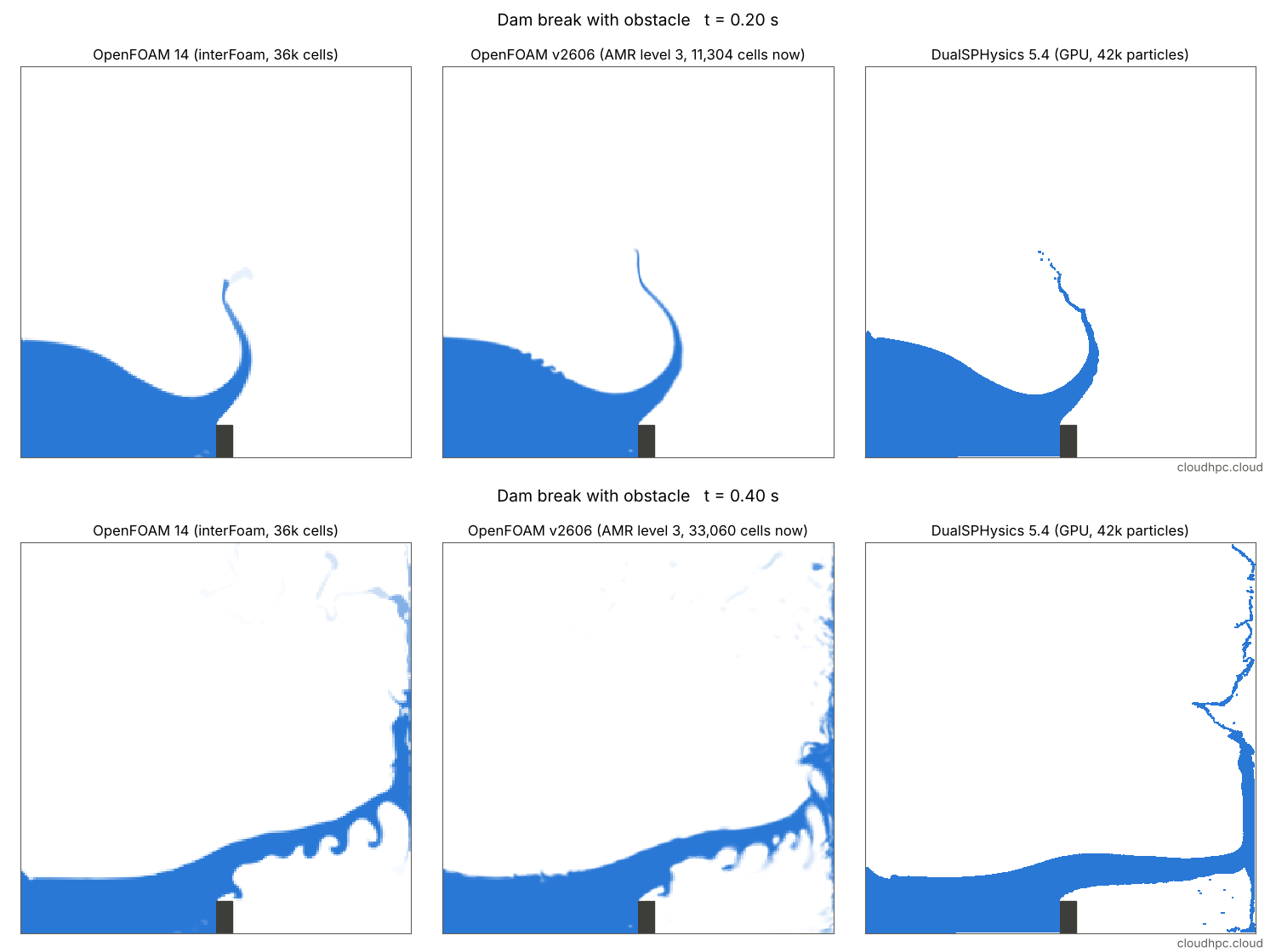
The dam break is the classic test for free-surface solvers. A column of water collapses, runs along the floor, hits an obstacle and then the opposite wall. It’s simple enough to run in minutes and violent enough to show how each method handles a breaking free surface.
We ran the same case with three solvers available on cloudHPC:
- OpenFOAM 14 (OpenFOAM Foundation),
interFoam-type VOF throughfoamRun - OpenFOAM v2606 (OpenCFD/Keysight),
interFoam, including adaptive mesh refinement (AMR) - DualSPHysics 5.4, a GPU-accelerated Smoothed Particle Hydrodynamics (SPH) code
The goal isn’t to crown a winner. We wanted to see how close two very different approaches (a fixed mesh with an interface-capturing scheme, and a meshless particle method) come on identical geometry, and what each costs on the cloud.

1. The case
The geometry is the OpenFOAM damBreak tutorial, a 2D tank 0.584 m × 0.584 m:
- Water column 0.146 m wide and 0.292 m high against the left wall
- Obstacle 0.024 m wide and 0.048 m high on the floor, at x = 0.292 m
- 1 s of physical time; water and air for OpenFOAM, water only for DualSPHysics
We built the DualSPHysics case with the same dimensions, starting from the 2D dam-break validation example shipped with DualSPHysics.
Resolutions
| Solver | Runs |
|---|---|
| OpenFOAM 14 and v2606 | Uniform meshes of 2,268 (tutorial), 7,700, 36,288 and 145,152 cells |
| OpenFOAM v2606 | AMR on alpha.water with 2 and 3 refinement levels, starting from the tutorial mesh |
| OpenFOAM 14 | AMR with 2 refinement levels (level 3 still running at the time of writing) |
| DualSPHysics | Particle spacing of 2, 1 and 0.5 mm, i.e. about 10.7k, 42.6k and 170k particles |
All OpenFOAM runs used highcore machines (physical cores only) on spot instances. DualSPHysics ran on a single NVIDIA Tesla T4 GPU.
2. What we compared
We used four quantities, computed in the same way for all three codes:
- Front position: the furthest point the water reaches within 10 mm of the floor, before the obstacle.
- Water extent: the x position reached by 99% of the water. This is more robust than the tip after the flow jumps the obstacle.
- Water height at the left wall: how fast the column drains.
- Water conservation: total water area over time.
For the front position we also have an experimental reference: the dam-break measurements of Koshizuka & Oka (1996), which use the same column size (0.146 m × 0.292 m) but no obstacle. So the comparison with the experiment is valid only until the water reaches the obstacle, at about 0.13–0.15 s.
A note on terms. Comparing with the experiment is a (limited) validation: are we solving the right equations for this physics? Refining the mesh and the particle spacing is a verification exercise: are we solving the equations accurately enough? We did both, on a small scale.
3. Results
Front position and water extent

- The three codes agree closely. Before the obstacle the fronts are within about 6 mm of each other. All three reach the obstacle face between 0.12 and 0.15 s.
- The simulations run ahead of the experiment. At t = 0.10 s they give 0.25 m against 0.21 m measured, and the experiment reaches the obstacle position at about 0.15 s. In a dam-break experiment the water is released by removing a gate, which takes a finite time, while the simulations release the column instantly; this is the usual explanation for a time offset of this kind. Once shifted by about 0.02 s, the simulated fronts follow the slope of the measurements.
- After the obstacle the water extent curves stay within 1–2 cm of each other until the flow reaches the right wall at about 0.33 s.
Draining of the column
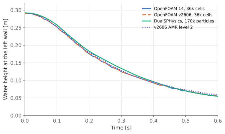
The column drains in almost exactly the same way in all codes. DualSPHysics is 5–10 mm higher between 0.15 and 0.35 s. After about 0.6 s the reflected wave returns to the left wall as a mix of jets and droplets, and a single “height” stops being meaningful. That’s why the plot stops there.
Effect of resolution
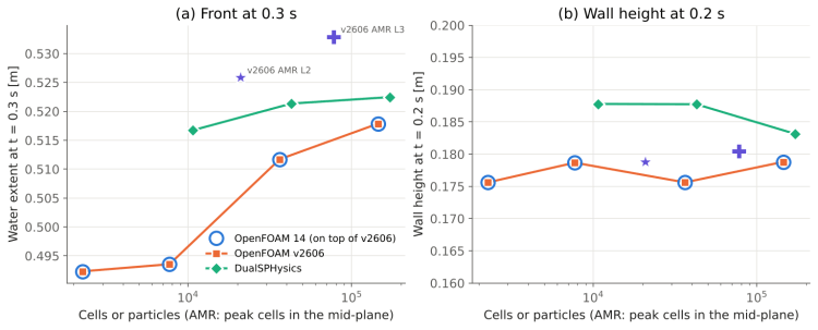
- OpenFOAM 14 and OpenFOAM v2606 give the same answer on the same mesh, down to the millimetre on the three finer uniform meshes (on the coarse tutorial mesh they differ by up to 1.5 cm during the impact on the obstacle). The two branches have diverged in many areas, but for this classic VOF case they behave identically.
- With refinement, the OpenFOAM water extent at 0.3 s moves from 0.492 m (tutorial mesh) to 0.518 m (145k cells). DualSPHysics moves from 0.517 m to 0.522 m. The two methods converge towards each other.
- AMR gives a result consistent with the finest uniform meshes (0.526 m at level 2, 0.533 m at level 3) with far fewer cells. Part of the small offset comes from the initial condition: with AMR the water column is set on the coarse tutorial mesh, so the initial water area is about 4% larger.
Water conservation
Up to 0.3 s, water is conserved to better than 0.1% in all runs. Between 0.3 and 0.5 s the jet hits the right wall and runs up it; some spray leaves through the open top. Over the full second, the uniform OpenFOAM runs lose about 1.7–2% of the water and DualSPHysics about 1% (particles leaving the domain). This is physical outflow through the open boundary, not a numerical leak.
The late, chaotic phase

The snapshots and the animation show the main qualitative difference between the methods. After the wave breaks:
- VOF (OpenFOAM) spreads the interface over a few cells, so jets and droplets become blurred regions of partially filled cells. AMR keeps them much sharper.
- SPH (DualSPHysics) keeps every fragment as a set of particles, with a sharp surface, but thin jets break into isolated particles once they get thinner than a few particle spacings.
Neither is “right” here: the real flow at this stage is 3D and turbulent, and a 2D simulation can only show its large-scale features.
4. Run time and cost
| Run | Cells / particles | Hardware | Solver time | Cost |
|---|---|---|---|---|
| OpenFOAM 14, tutorial mesh | 2,268 | 2 cores | 5 s | €0.017 |
| OpenFOAM 14 | 7,700 | 2 cores | 27 s | €0.017 |
| OpenFOAM 14 | 36,288 | 2 cores | 7.4 min | €0.032 |
| OpenFOAM 14 | 145,152 | 4 cores | 53 min | €0.207 |
| OpenFOAM v2606, tutorial mesh | 2,268 | 2 cores | 4 s | €0.017 |
| OpenFOAM v2606 | 7,700 | 2 cores | 28 s | €0.017 |
| OpenFOAM v2606 | 36,288 | 2 cores | 8.2 min | €0.033 |
| OpenFOAM v2606 | 145,152 | 4 cores | 61 min | €0.236 |
| OpenFOAM 14, AMR level 2 | up to ~86k (3D cells) | 2 cores | 49 min | €0.106 |
| OpenFOAM v2606, AMR level 2 | up to ~21k (mid-plane) | 2 cores | ~49 min (job) | €0.081 |
| OpenFOAM v2606, AMR level 3 | up to ~78k (mid-plane) | 4 cores | ~5.9 h (job) | €1.17 |
| DualSPHysics, 2 mm | 10,658 | 1 T4 GPU | 26 s | €0.366 for |
| DualSPHysics, 1 mm | 42,632 | 1 T4 GPU | 74 s | all three |
| DualSPHysics, 0.5 mm | 170,528 | 1 T4 GPU | 7.1 min | (one job) |
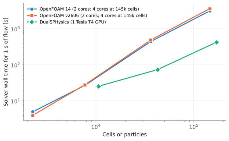
Costs are the actual amounts billed by cloudHPC on spot instances. For the smallest cases the cost is mostly machine start-up and data transfer, not computation.
What the numbers say:
- The whole uniform-mesh study, 8 OpenFOAM runs, cost about €0.58. The three DualSPHysics resolutions together cost €0.37.
- At similar model size the GPU wins. DualSPHysics with 170k particles took 7 minutes on one T4. OpenFOAM with 145k cells took about an hour on 4 CPU cores. SPH needs smaller time steps, but explicit particle updates map very well onto a GPU.
- AMR is not automatically cheaper here. The mesh changes at every time step and in this case the interface fills a large part of the domain after the wave breaks. Level 2 is a good trade-off, while level 3 cost more than the 145k-cell uniform mesh. AMR pays off when the interface occupies a small fraction of a large domain, which is the usual situation in engineering cases.
5. Takeaways
- For the global behaviour of a dam break (front speed, column draining, impact on the obstacle and the far wall), OpenFOAM VOF and DualSPHysics SPH agree within a few percent once the resolution is adequate.
- OpenFOAM 14 and OpenFOAM v2606 are interchangeable for this kind of case. Choose the branch for the other features you need.
- The tutorial mesh is too coarse for quantitative results. It gets the front about 2.5 cm (5%) behind at 0.3 s. Four times finer in each direction is enough for engineering accuracy here.
- DualSPHysics on a GPU is very fast for violent free-surface flows and naturally keeps fragments sharp. OpenFOAM gives more control over the mesh, the physics and the coupling with other models.
- On cloudHPC the whole study cost about €2.30, including the AMR runs, and every solver was already installed on the platform with no setup on our side.
All case files are available on request.
References
- S. Koshizuka, Y. Oka (1996). Moving-particle semi-implicit method for fragmentation of incompressible fluid. Nuclear Science and Engineering 123(3), 421–434. doi:10.13182/NSE96-A24205
- J. C. Martin, W. J. Moyce (1952). An experimental study of the collapse of liquid columns on a rigid horizontal plane. Phil. Trans. R. Soc. A 244, 312–324. doi:10.1098/rsta.1952.0006
- J. M. Domínguez et al. (2022). DualSPHysics: from fluid dynamics to multiphysics problems. Computational Particle Mechanics 9, 867–895. doi:10.1007/s40571-021-00404-2
- OpenFOAM Foundation, openfoam.org; OpenCFD/Keysight, openfoam.com; DualSPHysics, dual.sphysics.org
CloudHPC is a HPC provider to run engineering simulations on the cloud. CloudHPC provides from 1 to 224 vCPUs for each process in several configuration of HPC infrastructure - both multi-thread and multi-core. Current software ranges includes several CAE, CFD, FEA, FEM software among which OpenFOAM, FDS, Blender and several others.
New users benefit of a FREE trial of 300 vCPU/Hours to be used on the platform in order to test the platform, all each features and verify if it is suitable for their needs


