Wave propagation over a submerged bar: XBeach vs SWAN vs TELEMAC-3D on cloudHPC

Why a submerged bar?

When waves travel over a submerged bar, they steepen on the up-slope, release higher harmonics on the crest and then decompose into several free waves on the down-slope. A single sinusoid entering the flume leaves the bar as a jumble of components with different speeds. That makes the case a tough test of two things every coastal model must get right: frequency dispersion (how speed depends on wave length) and non-linear energy transfer between harmonics.

The Beji & Battjes (1993) experiments, run in a wave flume at Delft University of Technology, are one of the standard benchmarks for this: the measured time series of the 8 wave gauges are public (Mendeley Data, CC BY 4.0), so anyone can reproduce the comparison. We used them to verify three solvers that are less common on cloudHPC than OpenFOAM or FDS — and, in the process, to debug how cloudHPC runs them.

The three codes represent three different families:

• XBeach (Deltares) in non-hydrostatic mode: a depth-averaged, phase-resolving model with an extra layer for dispersion (de Ridder et al., 2021).
• SWAN (TU Delft): a spectral, phase-averaged model; it predicts wave energy, not the individual waves, and models non-linear transfer with a parametrised triad term.
• TELEMAC-3D (openTELEMAC consortium) in non-hydrostatic mode: a 3D finite-element model with 10 vertical levels, the most expensive of the three.

Results at a glance

Test	Metric (mean over 8 gauges)	XBeach 1.24	SWAN 41.51	TELEMAC-3D v8p5r1
SLN regular, non-breaking	|error| 1st / 2nd / 3rd harmonic	8.8 / 9.5 / 13.4 %	–	5.3 / 7.4 / 14.9 %
SLS, SLP regular, breaking	|error| 1st harmonic	11.9 %, 11.0 %	–	6.3 %, 2.7 %
SSN regular, short period	|error| 1st / 2nd / 3rd harmonic	7.7 / 23.6 / 40.6 %	–	2.8 / 31.5 / 50.9 %
JLN random, long period	|Hm0 error|, full record	2.7 %	3.4 %	3.3 % (10–150 s)
JSN random, short period	|Hm0 error|, full record	12.0 %	5.9 %	1.6 % (10–150 s)
All 6 random cases	|Hm0 error| range	2.3–12.0 %	1.6–5.9 %	1.6–3.3 % (2 cases)
Dispersion, kh = 0.5–3	phase speed error	+0.4 to +1.8 % (2 layers)	–	−0.3 to +0.02 %
Typical cost per run	billed, spot	€0.011 (regular), €0.03 (45 min random)	€0.02	€0.07 (60 s), €0.16–0.19 (200 s)

The experiment and how we set it up

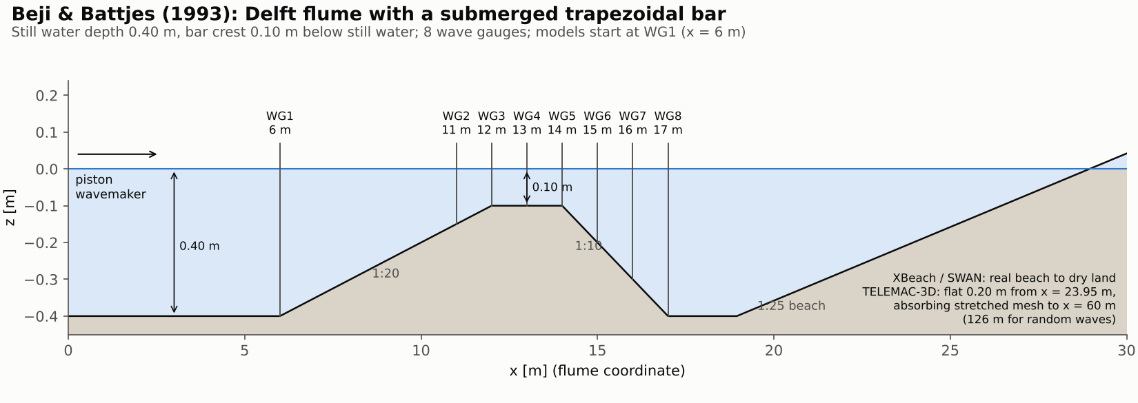
Figure 1 – The Delft flume: 0.40 m still water depth, a trapezoidal bar (1:20 up-slope, 2 m crest 0.10 m below still water, 1:10 down-slope) and a 1:25 beach. Wave gauge positions WG1–WG8 are those of the data set.

Wave conditions. Each regular case is named after its period and breaking type: SL = 2.5 s nominal period, SS = 1.0 s; N = non-breaking, S = spilling, P = plunging. The random cases JL* and JS* use JONSWAP spectra with the same peak periods. The regular records last 5 min, the random ones 45 min, sampled at 10 Hz. From the measured WG1 signal we found the true paddle frequency: 0.3959 Hz (T = 2.526 s) for the SL cases and 0.9897 Hz for the SS cases; six harmonics explain 99.88 % of the WG1 variance in SLN.

Boundary condition: the measured signal at WG1. None of the models starts at the paddle. All three are forced at x = 6 m (WG1) with the measured free surface:

• XBeach: the WG1 time series (filtered at 3 Hz) with the depth-averaged velocity from linear theory, wbctype = ts_nonh, weakly-reflective boundary (ARC = 1), real beach to dry land at the end, 1D grid with Δx = 0.02 m (1200 cells), CFL 0.7.
• SWAN: stationary 1D run; the incoming spectrum is the measured WG1 spectrum (Welch, 1024 points), triads (LTA) and depth-induced breaking on, 36 directional bins over ±45°, 60 frequencies between 0.1 and 3 Hz.
• TELEMAC-3D: non-hydrostatic, 10 levels, numerics taken from the openTELEMAC NonLinearWave validation case (Dingemans bar). A user routine imposes free surface, velocity profile and dynamic pressure from linear theory, per Fourier component. Regular cases: 4 harmonics fitted to WG1 (2 for SS). Random cases: the full WG1 record read from a formatted data file (FORMATTED DATA FILE 1). Triangular strip mesh with Δx = 0.02 m up to x = 30 m, then stretched to absorb the waves (to 60 m; 126 m for random waves); 4,554 nodes per level (5,001 for the random-wave mesh), Δt = 0.005 s (0.0025 s for SS).

The records start with the wave field already established, so the models start from rest with a cosine ramp; model time equals record time.

Metrics. For regular waves we fitted the amplitudes of the first three harmonics by least squares over 8 exact wave periods ending at 60 s. For the SS cases the TELEMAC-3D runs stopped early (see “What didn’t work”), so the window ends at 56 s (SSN), 55 s (SSS) and 53 s (SSP), for all models and the measurements. For random waves we compare Hm0 = 4σ. XBeach and SWAN use the whole 45-minute record. TELEMAC-3D was run for 200 s and compared over 10–150 s, before any reflection from the far end can return. Measurements are always taken over the same window as the model.

Regular waves: the bar releases higher harmonics

Case SLN (non-breaking, T = 2.53 s)

Figure 2 – First three harmonic amplitudes at the 8 gauges, measured (black) vs XBeach (blue) and TELEMAC-3D (orange). The grey band is the bar crest.

Gauge	x [m]	Measured A1 / A2 / A3 [cm]	XBeach error [%]	TELEMAC-3D error [%]
WG1	6	1.095 / 0.118 / 0.063	−6.4 / −27.4 / −0.4	+0.2 / +1.4 / +10.0
WG2	11	1.245 / 0.260 / 0.138	+10.5 / +26.0 / +2.5	+7.4 / +12.7 / +19.1
WG3	12	1.361 / 0.465 / 0.196	−6.0 / +9.7 / +45.5	−3.3 / +6.2 / +36.6
WG4	13	1.154 / 0.568 / 0.426	−11.7 / −1.6 / +5.0	−4.6 / +4.5 / +3.3
WG5	14	0.912 / 0.551 / 0.523	+1.5 / −1.8 / +19.1	+5.1 / +8.6 / +20.3
WG6	15	0.703 / 0.570 / 0.751	+11.9 / −1.9 / +11.8	+9.3 / +7.0 / +13.4
WG7	16	0.714 / 0.586 / 0.912	−13.5 / −5.1 / +8.4	−4.9 / +8.7 / +5.3
WG8	17	0.623 / 0.671 / 0.775	+8.9 / −2.4 / +14.1	+7.7 / +10.4 / +11.1
Mean |error|			8.8 / 9.5 / 13.4	5.3 / 7.4 / 14.9

Behind the bar (WG6–WG8) the third harmonic is as large as the first. Both phase-resolving models capture this energy transfer. The time series show it directly: at WG8 a single 2.5 s wave has become two crests per period, and both models follow the measured shape closely.

Figure 3 – Free-surface elevation on the bar crest (WG4) and behind it (WG6, WG8), 50–58 s.

All six regular cases

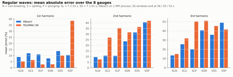
Figure 4 – Mean |error| over the 8 gauges for the first three harmonics.

Case	XBeach A1 / A2 / A3 [%]	TELEMAC-3D A1 / A2 / A3 [%]
SLN (non-breaking)	8.8 / 9.5 / 13.4	5.3 / 7.4 / 14.9
SLS (spilling)	11.9 / 10.8 / 25.5	6.3 / 26.9 / 31.9
SLP (plunging)	11.0 / 10.6 / 19.9	2.7 / 35.3 / 50.2
SSN (non-breaking, T = 1.01 s)	7.7 / 23.6 / 40.6	2.8 / 31.5 / 50.9
SSS (spilling)	13.7 / 31.4 / 35.8	10.0 / 36.3 / 45.3
SSP (plunging)	10.4 / 40.6 / 48.9	38.5 / 41.8 / 41.5

What we learned

• First harmonic: TELEMAC-3D is the most accurate in 5 of 6 cases (2.7–10.0 %). The exception is SSP, the plunging short-period case, where it overestimates the first harmonic by 53–80 % from the end of the crest onwards (WG5–WG8).
• Long-period breaking cases (SLS, SLP): TELEMAC-3D has no wave-breaking model in this set-up, so it overestimates the higher harmonics behind the bar (WG6–WG8: +56 % and +39 % on A2/A3 in SLS, +79 % and +84 % in SLP); mean A2 error over all gauges 27–35 % vs 11 % for XBeach, whose hydrostatic-front breaking treatment (Smit et al., 2013) keeps the energy at the right level.
• Short-period cases (SS): the 2nd and 3rd harmonics (2–3 Hz) are only 0.18–0.40 m long. Behind the bar both models lose a large part of them: 30–93 % at some gauges. This is a resolution limit: two layers in XBeach, 10 levels and a 2 cm mesh in TELEMAC-3D. Neither code is wrong here; the set-up is too coarse for those wave lengths.
• XBeach variants for SLN: a one-layer model gave 10.3 / 8.2 / 38.3 %. Forcing with the first harmonic only, instead of the measured signal, gave 9.9 / 18.8 / 31.3 %. The full two-layer set-up with measured forcing is the best overall, especially on the third harmonic (8.8 / 9.5 / 13.4 %).

Random waves: SWAN is hard to beat on Hm0

Figure 5 – Mean |Hm0 error| over the 8 gauges for the six JONSWAP cases.

Case	XBeach	SWAN	TELEMAC-3D (10–150 s)	XBeach over 10–150 s
JLN	2.7 %	3.4 %	3.3 %	1.4 %
JLS	2.3 %	3.4 %	–	–
JLP	3.5 %	2.5 %	–	–
JSN	12.0 %	5.9 %	1.6 %	12.2 %
JSS	7.3 %	1.6 %	–	–
JSP	5.8 %	1.9 %	–	–

What we learned

• SWAN is within 11 % at every gauge in every case and costs €0.02 per run. If what you need is the wave height distribution over a bar, a phase-averaged model is the right tool. Its main bias is +5 to +9 % on the bar crest (WG4–WG5) in four of the six cases (JL*, JSN), from the parametrised triads. The mean period follows the harmonic release reasonably: in JLN the measured Tm01 drops from 1.67 s at WG1 to 1.06 s at WG8, SWAN gives 0.97 s (−9 %).
• XBeach matches SWAN for long-period waves, but is about 10 % low already at WG1 for the short-period JS* cases. That points to energy lost at the inlet for the high-frequency part of the spectrum, an open point of our set-up.
• TELEMAC-3D reads the measured inlet series correctly in parallel. In JSN it gives the lowest error of the three (1.6 %), at the highest cost: €0.16–0.19 for 200 s on 8 cores, against €0.03 for 45 minutes of XBeach.

Dispersion check: are the models fast enough?

Before trusting harmonics we tested each model alone: a flat channel (h = 0.40 m), a sinusoid of 0.5 cm amplitude at kh = 0.5, 1, 2 and 3, phase speed fitted between x = 1 and 9 m.

Figure 6 – Phase speed and wave height error vs linear theory.

kh	TELEMAC-3D speed / height	XBeach 2 layers speed / height	XBeach 1 layer speed / height
0.5	+0.02 % / −0.6 %	+0.46 % / −1.0 %	−0.08 % / −0.8 %
1.0	−0.14 % / +0.8 %	+1.35 % / −1.2 %	−1.31 % / +0.4 %
2.0	−0.31 % / +9.8 %	+1.84 % / −7.2 %	−14.2 % / −17.4 %
3.0	−0.23 % / +31.6 %	+0.41 % / −21.0 %	wave does not propagate

Both phase-resolving models get the speed right well beyond the kh ≈ 1.7 of the SS cases. The height drifts at high kh in opposite directions: XBeach damps the wave, while in TELEMAC-3D it ends up as much as 32 % higher than the input. The TELEMAC-3D growth is most likely a mismatch of our linear-theory inlet condition for short waves (open point). The one-layer XBeach model behaves exactly as its theory says: fine up to kh ≈ 1, wrong at kh = 2.

What didn’t work (and what we changed on cloudHPC)

This benchmark was also a debugging exercise for the cloudHPC launchers. In the order we met them:

1. XBeach non-hydrostatic on several MPI processes. On a 4 vCPU machine the launcher split the 1D grid over 3 processes. With wavemodel = nonh the free surface jumped at the subdomain boundaries before any wave had arrived: 3.1 cm at x = 16.84 m after 1 s (and about 8 cm after 4 s) in the one-layer dispersion case, about 0.6 cm (as large as the incident wave) with two layers. With one layer the wave speed came out +42 % to +460 % wrong. With two layers it polluted the higher harmonics: the third harmonic at WG1 in SLN came out +212 % instead of −0.4 %.

Figure 7 – Left: spurious waves at the subdomain boundaries (3 processes) vs a flat surface (1 process). Right: SLN third harmonic, 3 vs 1 process.

We reran all 22 XBeach cases on a single process (€0.36 in total); every XBeach number in this post comes from those runs. 1D cases take from a few seconds to about 15 minutes of solver time on one core, so nothing is lost. The cloudHPC XBeach launcher now runs non-hydrostatic cases on one process and prints a warning if more are requested.

2. TELEMAC-3D launcher and image. The first launcher stripped the .cas extension (“Could not find your steering file”). The shared build could not find its own libraries (libbief4partel.so, then libmed.so.11). The new Ubuntu 24.04 image needed med_parameter.hf, which the Ubuntu MED package does not ship. All fixed: the image registers its libraries with ldconfig, and the launcher now detects the module, the configuration and missing libraries by itself.

3. TELEMAC-3D short-period cases stopped between t ≈ 53 and 57 s with CALCOT: PLANES 1 AND 2 INTERCROSS: the depth went negative at the far end wall, 43 m beyond the last gauge, where the stretched mesh is too coarse for 1 Hz waves. Nothing from there can reach the gauges before 60 s, so we used the partial results written by each process, with fit windows ending just before each stop (53–56 s). Lesson: on cloudHPC the useful TELEMAC message is in the per-process PE*.LOG files, not at the end of the main log.

4. XBeach sloshing test dropped. We first tried a standing wave in a closed basin to check dispersion. XBeach takes zsinitfile as the reference water level, not as an initial disturbance, so the basin never sloshed. We replaced it with the linear dispersion test above.

5. SWAN stops on a title line longer than allowed and on COMPUTE STATIONARY in a stationary run. Both errors appear only in the .erf/.prt files while the run reports “Normal end”.

Run times and costs

All runs on cloudHPC spot instances; costs are the billed amounts (boot, run, upload).

Run type	Instance	Solver time	Billed cost
XBeach, regular case, 60 s	2 vCPU highcore, 1 process	≤ 12 s	€0.011
XBeach, random case, 45 min	2 vCPU highcore, 1 process	~11–14 min	€0.029–0.034
SWAN, stationary 1D	4 vCPU highcpu	< 1 min	€0.017–0.019
TELEMAC-3D, regular case, 60 s	4 vCPU highcore	8 min 24 s (SLN)	€0.069–0.076
TELEMAC-3D, random case, 200 s	8 vCPU highcore	16 min 48 s (JLN)	€0.160–0.188
TELEMAC-3D, dispersion, 4 cases	4 vCPU highcore	–	€0.094
Whole study	69 runs incl. tests and reruns		€2.29

How to run these cases on cloudHPC

1. Upload one folder per case (the cases/ folder of the download contains them all):
   • XBeach: params.txt, x.grd, bed.dep, boun_U.bcf. Launch XBeach_mpi with 2 vCPU highcore.
   • SWAN: .swn, bed.dep, wg1.sp1, gauges.loc. Launch SWAN-41.51 with 4 vCPU highcpu.
   • TELEMAC-3D: .cas, geo_bb93.slf, geo_bb93.cli, user_bb93.f and, for random waves, bb93_bc.txt. Launch openTELEMAC-v8p5r1 with 4–8 vCPU highcore. Several .cas files in one folder run one after the other.
2. XBeach non-hydrostatic: keep it on one process (2 vCPU). Check XBlog.txt: it must say “running on 1 processes”.
3. SWAN: read the .prt file; a run can end “normally” with an error in it.
4. TELEMAC-3D: with a FORTRAN FILE, keep variable names short (72-column fixed form) and avoid names used by BIEF routines (we hit OM). If a run stops, read PE*.LOG in the working folder.
5. Storage is kept for 60 days: download what you need.

FAQ

Which model should I use for waves over a bar or reef?
For wave heights and set-up over large areas: SWAN — 1.6–5.9 % mean Hm0 error here, cents per run. For wave shapes, harmonics, run-up or overtopping: a phase-resolving model. XBeach non-hydrostatic is cheap and good for long-period waves; TELEMAC-3D is the most accurate on the first harmonic but costs about 6× more per run; XBeach does better on the higher harmonics when waves break.

Is XBeach non-hydrostatic accurate for dispersive waves?
With two layers, yes: the phase speed was within 1.9 % of linear theory up to kh = 3 in our test. With one layer it is fine up to kh ≈ 1.

Can I run XBeach non-hydrostatic in parallel?
In our tests (XBeach 1.24.6170M, 1D grid) running on more than one MPI process created spurious waves at the subdomain boundaries. Run 1D non-hydrostatic cases on one process; on cloudHPC the launcher now does this for you.

Does TELEMAC-3D need a wave-breaking model for this case?
For the long-period spilling and plunging cases (SLS, SLP), yes: without one, the higher harmonics behind the bar are overestimated by 39–84 %.

How much does it cost to run this benchmark in the cloud?
On cloudHPC a single XBeach or SWAN run costs about €0.01–0.03, a TELEMAC-3D run €0.07–0.19. The full study (69 runs, including tests and reruns) cost €2.29.

References

1. Beji, S., & Battjes, J. A. (1993). Experimental investigation of wave propagation over a bar. Coastal Engineering, 19(1–2), 151–162. https://doi.org/10.1016/0378-3839(93)90022-Z
2. Beji, S. (2017). Delft Experiments Data 1993 Paper (Version 1) [Data set]. Mendeley Data, CC BY 4.0. https://doi.org/10.17632/7x2y76mkjs.1
3. Smit, P., Zijlema, M., & Stelling, G. (2013). Depth-induced wave breaking in a non-hydrostatic, near-shore wave model. Coastal Engineering, 76, 1–16. https://doi.org/10.1016/j.coastaleng.2013.01.008
4. de Ridder, M. P., et al. (2021). Efficient two-layer non-hydrostatic wave model with accurate dispersive behaviour. Coastal Engineering. TU Delft repository: https://repository.tudelft.nl/record/uuid:2025fc04-5e7e-4509-8834-3eb3b19f1ae9
5. Booij, N., Ris, R. C., & Holthuijsen, L. H. (1999). A third-generation wave model for coastal regions: 1. Model description and validation. Journal of Geophysical Research: Oceans, 104(C4), 7649–7666. https://doi.org/10.1029/98JC02622
6. XBeach documentation: https://xbeach.readthedocs.io
7. SWAN: https://swanmodel.sourceforge.io
8. openTELEMAC (v8p5r1, examples/telemac3d/NonLinearWave): https://gitlab.pam-retd.fr/otm/telemac-mascaret

---

CloudHPC is a HPC provider to run engineering simulations on the cloud. CloudHPC provides from 1 to 224 vCPUs for each process in several configuration of HPC infrastructure - both multi-thread and multi-core. Current software ranges includes several CAE, CFD, FEA, FEM software among which OpenFOAM, FDS, Blender and several others.

New users benefit of a FREE trial of 300 vCPU/Hours to be used on the platform in order to test the platform, all each features and verify if it is suitable for their needs

---

Contact Name/Surname *

Company Name *

Company address *

City *

State/Province *

Country *CountryArubaAfghanistanAngolaAnguillaÅland IslandsAlbaniaAndorraUnited Arab EmiratesArgentinaArmeniaAmerican SamoaAntarcticaFrench Southern TerritoriesAntigua and BarbudaAustraliaAustriaAzerbaijanBurundiBelgiumBeninBonaire, Sint Eustatius and SabaBurkina FasoBangladeshBulgariaBahrainBahamasBosnia and HerzegovinaSaint BarthélemyBelarusBelizeBermudaBolivia, Plurinational State ofBrazilBarbadosBrunei DarussalamBhutanBouvet IslandBotswanaCentral African RepublicCanadaCocos (Keeling) IslandsSwitzerlandChileChinaCôte d'IvoireCameroonCongo, The Democratic Republic of theCongoCook IslandsColombiaComorosCabo VerdeCosta RicaCubaCuraçaoChristmas IslandCayman IslandsCyprusCzechiaGermanyDjiboutiDominicaDenmarkDominican RepublicAlgeriaEcuadorEgyptEritreaWestern SaharaSpainEstoniaEthiopiaFinlandFijiFalkland Islands (Malvinas)FranceFaroe IslandsMicronesia, Federated States ofGabonUnited KingdomGeorgiaGuernseyGhanaGibraltarGuineaGuadeloupeGambiaGuinea-BissauEquatorial GuineaGreeceGrenadaGreenlandGuatemalaFrench GuianaGuamGuyanaHong KongHeard Island and McDonald IslandsHondurasCroatiaHaitiHungaryIndonesiaIsle of ManIndiaBritish Indian Ocean TerritoryIrelandIran, Islamic Republic ofIraqIcelandIsraelItalyJamaicaJerseyJordanJapanKazakhstanKenyaKyrgyzstanCambodiaKiribatiSaint Kitts and NevisKorea, Republic ofKuwaitLao People's Democratic RepublicLebanonLiberiaLibyaSaint LuciaLiechtensteinSri LankaLesothoLithuaniaLuxembourgLatviaMacaoSaint Martin (French part)MoroccoMonacoMoldova, Republic ofMadagascarMaldivesMexicoMarshall IslandsNorth MacedoniaMaliMaltaMyanmarMontenegroMongoliaNorthern Mariana IslandsMozambiqueMauritaniaMontserratMartiniqueMauritiusMalawiMalaysiaMayotteNamibiaNew CaledoniaNigerNorfolk IslandNigeriaNicaraguaNiueNetherlandsNorwayNepalNauruNew ZealandOmanPakistanPanamaPitcairnPeruPhilippinesPalauPapua New GuineaPolandPuerto RicoKorea, Democratic People's Republic ofPortugalParaguayPalestine, State ofFrench PolynesiaQatarRéunionRomaniaRussian FederationRwandaSaudi ArabiaSudanSenegalSingaporeSouth Georgia and the South Sandwich IslandsSaint Helena, Ascension and Tristan da CunhaSvalbard and Jan MayenSolomon IslandsSierra LeoneEl SalvadorSan MarinoSomaliaSaint Pierre and MiquelonSerbiaSouth SudanSao Tome and PrincipeSurinameSlovakiaSloveniaSwedenEswatiniSint Maarten (Dutch part)SeychellesSyrian Arab RepublicTurks and Caicos IslandsChadTogoThailandTajikistanTokelauTurkmenistanTimor-LesteTongaTrinidad and TobagoTunisiaTürkiyeTuvaluTaiwan, Province of ChinaTanzania, United Republic ofUgandaUkraineUnited States Minor Outlying IslandsUruguayUnited StatesUzbekistanHoly See (Vatican City State)Saint Vincent and the GrenadinesVenezuela, Bolivarian Republic ofVirgin Islands, BritishVirgin Islands, U.S.Viet NamVanuatuWallis and FutunaSamoaYemenSouth AfricaZambiaZimbabwe

Company address Privacy

Email *

Email

Confirm Email

Privacy *

• I accept the privacy conditions

Privacy Policy

Send registration