Palabos vs OpenFOAM on cloudHPC: lattice Boltzmann and finite volume on two classic benchmarks
TL;DR
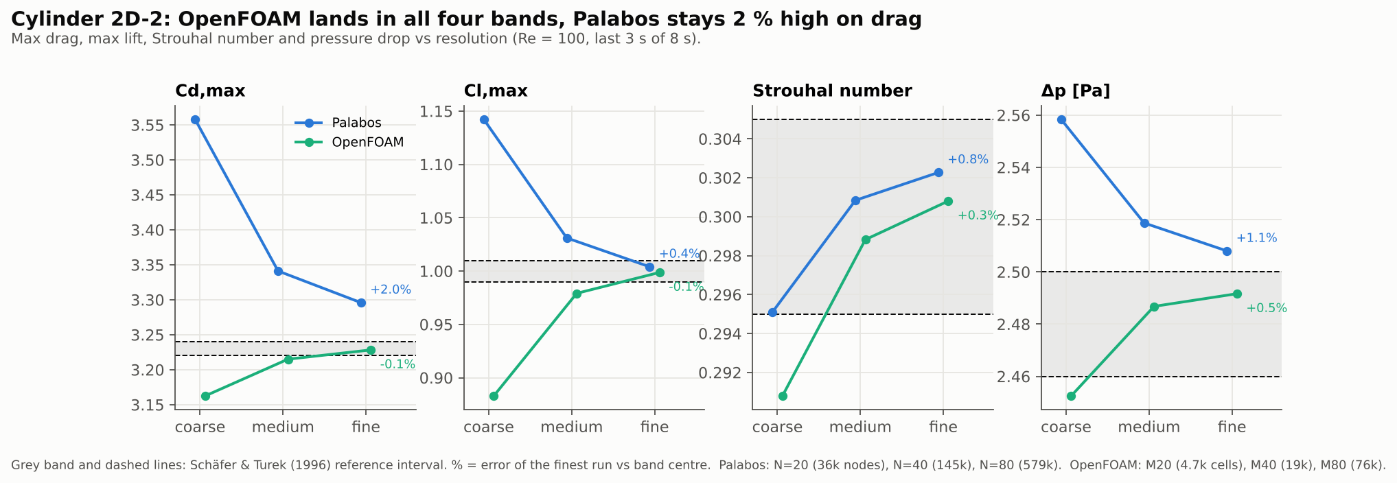
- Cylinder at Re = 100 (Schäfer–Turek 2D-2): both codes converge to the reference values. OpenFOAM lands inside all four reference bands with only 76k cells (Cd,max 3.228, Cl,max 0.999, St 0.301). Palabos gets there in lift, Strouhal and Δp but stays +2 % on drag at 80 nodes per diameter because of its staircase cylinder wall.
- 3D Taylor–Green vortex at Re = 1600, 256³: Palabos reproduces the DNS dissipation rate within 1.0 % RMS (peak 0.01315 vs 0.01306); OpenFOAM is at 3.9 % and peaks early.
- Speed and cost (256³, 96 vCPU): Palabos 3.6 min / €3.47 vs OpenFOAM 85 min / €33.50: about 23× faster and 10× cheaper on the same grid.
- Scaling: Palabos goes from 23 min on 8 vCPU to 3.6 min on 96 vCPU (6.4× speed-up), but the cheapest run is the smallest machine (€0.90).
- Right tool for the job: curved walls and complex boundaries at modest cell counts → OpenFOAM. Large, mostly-fluid, unsteady domains where throughput is everything → lattice Boltzmann.

Why compare lattice Boltzmann and finite volume now
Lattice Boltzmann (LBM) codes are moving from research tools into engineering workflows: urban wind, data-centre cooling, porous media, biomedical flows. Their selling point is throughput: a simple, local update on a uniform grid that maps very well onto modern CPUs and GPUs. The question engineers ask us is practical: for the same physics, is an LBM code more accurate, faster, or cheaper than the finite-volume solver I already know?
We answered it on cloudHPC with two open-source codes:
- Palabos, the Parallel Lattice Boltzmann Solver from the University of Geneva (C++, MPI);
- OpenFOAM (ESI edition), the reference open-source finite-volume CFD toolbox.
A third code, OpenLB, was part of the plan. Its cases are ready, but its GPU build on cloudHPC needs a platform fix first; it will get its own follow-up post (see What we learned).
Results at a glance
| Case | Metric | Reference | Palabos (finest) | OpenFOAM (finest) |
|---|---|---|---|---|
| Cylinder 2D-2, Re = 100 | Cd,max | 3.22–3.24 | 3.296 (+2.0 %) | 3.228 |
| Cl,max | 0.99–1.01 | 1.004 | 0.999 | |
| Strouhal | 0.295–0.305 | 0.302 | 0.301 | |
| Δp [Pa] | 2.46–2.50 | 2.508 (+1.1 %) | 2.492 | |
| Taylor–Green 256³, Re = 1600 | Peak dissipation ε | 0.01306 at t = 8.94 | 0.01315 at t = 8.91 | 0.01179 at t = 8.40 |
| RMS error of ε(t) | — | 1.0 % | 3.9 % | |
| Solve time / cost, 96 vCPU | — | 217 s / €3.47 | 5105 s / €33.50 |
Bold = inside the reference band (cylinder) or best of the two (Taylor–Green).
How the runs were set up
- Solvers: Palabos (current release on cloudHPC, compiled automatically from our C++ program, MPI) and OpenFOAM ESI (latest release on cloudHPC,
pimpleFoam). - Hardware: cloudHPC hypercore instances (physical cores only, latest CPU generation). Validation runs on preemptible (spot) machines; all timing runs on regular instances, so no preemption could distort the times.
- No turbulence model anywhere: both codes solve the flow directly.
- Same lattice/grid parameters across resolutions: Palabos D2Q9/D3Q19 with acoustic scaling (lattice velocity of the mean inflow 0.05, Mach ≈ 0.09); OpenFOAM second-order in space (linear) and time (backward).
- All input files are available on request and the step-by-step setup is below.
Case 1: Schäfer–Turek 2D-2, unsteady flow around a cylinder

Setup. The DFG benchmark of Schäfer & Turek (1996): a 2.2 × 0.41 m channel, a cylinder of diameter 0.1 m slightly off the centreline, parabolic inflow with mean velocity 1 m/s, ν = 10⁻³ m²/s, so Re = 100. The flow sheds a regular von Kármán street. We measure maximum drag and lift coefficient, the Strouhal number and the pressure difference between the front and back of the cylinder, and compare them with the published reference intervals. Each run simulates 8 s and the metrics use the last 3 s.
- Palabos: regularized BGK, local velocity/pressure boundaries, cylinder as a staircase of bounce-back nodes with momentum-exchange force evaluation. Resolutions: 20, 40 and 80 nodes per diameter (36k to 579k nodes).
- OpenFOAM: structured O-grid built with
blockMesh(5k, 19k and 76k cells), parabolic inlet with thefixedProfileboundary condition,forceCoeffsandprobesfunction objects.
Results.

| Run | Size | Cd,max | Cl,max | St | Δp [Pa] | Machine | Cost |
|---|---|---|---|---|---|---|---|
| Palabos N = 20 | 36k nodes | 3.558 | 1.142 | 0.295 | 2.558 | hypercore 8, one job | €0.33 (all three) |
| Palabos N = 40 | 145k nodes | 3.341 | 1.031 | 0.301 | 2.519 | ||
| Palabos N = 80 | 579k nodes | 3.296 | 1.004 | 0.302 | 2.508 | ||
| OpenFOAM M20 | 4.7k cells | 3.162 | 0.883 | 0.291 | 2.453 | hypercore 2 | €0.08 |
| OpenFOAM M40 | 19k cells | 3.215 | 0.979 | 0.299 | 2.487 | hypercore 2 | €0.14 |
| OpenFOAM M80 | 76k cells | 3.228 | 0.999 | 0.301 | 2.492 | hypercore 2 | €0.53 |
| Reference (Schäfer & Turek) | 3.22–3.24 | 0.99–1.01 | 0.295–0.305 | 2.46–2.50 | |||
What we learned.
- Body-fitted meshes win on curved walls. OpenFOAM’s O-grid follows the cylinder exactly, so 76k cells are enough to sit inside every reference band. Palabos approaches the band from above and, at 80 nodes per diameter, still over-predicts peak drag by 2 %: the staircase wall makes the cylinder effectively a little larger. LBM codes offer curved (interpolated) wall treatments for exactly this reason; with them the error drops at much lower resolution. This is the point to check before choosing an LBM code for external aerodynamics.
- Watch the acoustics in LBM. Lattice Boltzmann is weakly compressible. Our first Palabos run started the inflow impulsively and excited the channel’s acoustic quarter-wave mode (about 1.3 Hz, the lattice speed of sound over four channel lengths), which polluted the drag signal. A smooth 2 s ramp of the inflow, as recommended in the LBM literature and in OpenLB’s own example, removed it. Finite-volume incompressible solvers do not have this issue.
- Throughput is already visible in 2D. Palabos ran the finest case (579k nodes, 128,000 time steps) in 3 minutes on 8 cores at 404 million lattice updates per second (MLUPS).
Case 2: 3D Taylor–Green vortex at Re = 1600

Setup. A periodic box [0, 2π]³ initialised with the Taylor–Green velocity and pressure fields (V₀ = 1 m/s, L = 1 m, ν = 1/1600 m²/s). The vortices stretch, break down into small-scale turbulence around t ≈ 9 and decay. We record the volume-averaged kinetic energy Eₖ every 0.05 s and compare its dissipation rate ε = −dEₖ/dt with the DNS of Brachet et al. (1983). There are no walls and no boundary conditions, so the comparison isolates the numerical method.
- Palabos: D3Q19, BGK collision (the regularized model was 7× slower in 3D for this case), consistent initial density from the analytical pressure.
- OpenFOAM:
pimpleFoam, cyclic patches, initial fields with#codeStream, fixed Δt (Courant ≈ 0.2), kinetic energy fromvolFieldValue. - Grids: 128³ (2.1 M) and 256³ (16.8 M) nodes/cells.
Accuracy.

| Grid | Code | Peak ε | at t | RMS error vs DNS |
|---|---|---|---|---|
| — | Brachet et al. DNS | 0.01306 | 8.94 | — |
| 128³ | Palabos | 0.01252 | 8.54 | 2.4 % |
| OpenFOAM | 0.01349 | 8.45 | 8.1 % | |
| 256³ | Palabos | 0.01315 | 8.91 | 1.0 % |
| OpenFOAM | 0.01179 | 8.40 | 3.9 % |
Speed, scaling and cost (256³).

| Code | vCPU | Solve time | Throughput | Speed-up vs 8 vCPU | Parallel efficiency | Billed cost |
|---|---|---|---|---|---|---|
| Palabos | 8 | 1390 s | 98 MLUPS | 1.0× | 100 % | €0.90 |
| 16 | 944 s | 145 MLUPS | 1.5× | 74 % | €1.31 | |
| 32 | 532 s | 257 MLUPS | 2.6× | 65 % | €1.87 | |
| 48 | 333 s | 411 MLUPS | 4.2× | 70 % | €2.10 | |
| 96 | 217 s | 629 MLUPS | 6.4× | 53 % | €3.47 | |
| OpenFOAM | 32 | 13067 s | 6.53 s/step | 1.0× (vs 32) | 100 % | €27.03 |
| 48 | 10441 s | 5.22 s/step | 1.25× | 83 % | €32.39 | |
| 96 | 5105 s | 2.55 s/step | 2.56× | 85 % | €33.50 |
What we learned.
- On a periodic, fully resolved flow, LBM is both faster and closer to the DNS. At 256³ Palabos needs 3.6 minutes on 96 cores and matches the reference within 1 %. OpenFOAM needs 85 minutes on the same machine for a 3.9 % error. The difference is the algorithm: Palabos does one local, memory-bound update per node per step; OpenFOAM solves a pressure equation every step, and at 16.8 M cells the GAMG solver needs up to 25 iterations per final corrector.
- Palabos is memory-bandwidth bound. Doubling cores does not halve the time (53 % efficiency at 96 vCPU). Buy cores for turnaround, not for savings: the 8-vCPU run is the cheapest (€0.90), the 96-vCPU run the fastest (3.6 min).
- OpenFOAM scales well, so for it the big machine is nearly free. From 32 to 96 vCPU it runs 2.56× faster at 85 % efficiency, and the cost per run only rises from €27 to €34. From 48 to 96 vCPU it is 2.05× faster, slightly better than ideal.
- The pressure solver dominates the cost of finite-volume runs at this size. That is the honest price of an incompressible formulation, and also where OpenFOAM users can gain the most (solver settings, tolerances, time-step size).
Failures as they happened on cloudHPC
Benchmarks are only useful if they show what went wrong too.
- Impulsive start in Palabos (cylinder): acoustic standing wave in the drag signal, Cd,max too high at N = 40. Fix: 2 s cosine ramp of the inflow.
- Pressure probes on the wall: at (0.15, 0.2) and (0.25, 0.2) the probe falls on a solid bounce-back node in a staircase cylinder and returns Δp = 0. Fix: sample the first fluid node in front of and behind the cylinder.
- OpenFOAM
fixedProfilewith a vector polynomial: the exponent must be a vector too,((14.63 0 0) (1 1 1)), otherwise the case stops with Expected a ‘(‘ while reading VectorSpace. - OpenLB: the cloudHPC build is a CUDA build; on a CPU machine it stops with
libcuda.so.1: cannot open shared object file, and on the T4 GPU nodes it reported No CUDA device found. It is being fixed on the platform side; OpenLB results will follow in a separate post.
Run times and costs
| Batch | Runs | Instances | Cost |
|---|---|---|---|
| Cylinder 2D-2 | Palabos N20/40/80, OpenFOAM M20/40/80 | hypercore 8 and 2, spot | €1.08 |
| Taylor–Green 128³ | Palabos (8 vCPU), OpenFOAM (16 vCPU) | hypercore, spot | €0.96 |
| Taylor–Green 256³, Palabos | 8 / 16 / 32 / 48 / 96 vCPU | hypercore, regular | €9.65 |
| Taylor–Green 256³, OpenFOAM | 32 / 48 / 96 vCPU | hypercore, regular | €92.92 |
| Taylor–Green 256³, OpenFOAM | 16 vCPU, stopped to limit cost | hypercore, regular | €6.82 |
Billed costs include instance start-up, compilation (Palabos) and result upload, which is why short runs on large machines cost relatively more.
How to run these cases on cloudHPC
Palabos
- Put your C++ program (a
.cppwithmain()) and exactly one.xmlparameter file in a folder. To run several cases in one job, use one sub-folder per case: they run one after the other, each on all cores. - Your own
CMakeLists.txtis ignored: cloudHPC compiles the program against its Palabos build (C++17, optimised, MPI). Code that builds with the standard Palabos examples builds here too. - Pick hypercore or highcore (one MPI process per physical core). For 3D LBM, check the collision model’s speed first: in our test plain BGK ran at 25 MLUPS on two cores against 3.5 MLUPS for the regularized BGK.
- Logs:
log.compilefor compilation errors,log.<program>for the run.
OpenFOAM
- Upload a standard case (
0/,constant/,system/). Withoutconstant/polyMesh, cloudHPC runsblockMesh(or snappyHexMesh / cfMesh) automatically, thendecomposeParwith the right number of subdomains. #codeStreaminitial conditions and coded boundary conditions are compiled on the machine.- Use hypercore or highcore with at least ~50k cells per core; at 256³ the pressure solve dominates, so test solver tolerances before a long run.
- Results are reconstructed automatically and a
case.foamfile is created for ParaView.
Both: use regular instances for timing studies and spot instances for everything else; download your results, storage is cleaned after 60 days.
FAQ
Is lattice Boltzmann more accurate than finite volume?
Not in general. In our tests Palabos was more accurate on the periodic Taylor–Green vortex (1.0 % vs 3.9 % RMS error at 256³), while OpenFOAM was more accurate on the cylinder with fewer cells, because its body-fitted mesh represents the curved wall exactly.
How much faster is Palabos than OpenFOAM?
On the 256³ Taylor–Green vortex with 96 vCPU, Palabos solved in 217 s and OpenFOAM in 5105 s, about 23× faster, at roughly a tenth of the cost. The gap depends on the case: flows dominated by complex walls or needing local refinement narrow it.
Does Palabos scale well on cloud CPUs?
It scales, but it is memory-bandwidth bound: 6.4× speed-up from 8 to 96 vCPU (53 % efficiency). The smallest machine gives the lowest cost per run, larger machines the shortest turnaround.
Why did the LBM drag oscillate at the start of the cylinder run?
LBM is weakly compressible: an impulsive inflow launches pressure waves that resonate in the channel. A smooth ramp of the inflow over a few flow-through times removes them.
Can I run OpenLB on cloudHPC?
OpenLB is installed as a GPU (CUDA) build. A platform issue currently prevents it from running; the OpenLB part of this comparison will be published as soon as it is fixed.
References
- M. Schäfer, S. Turek, Benchmark Computations of Laminar Flow Around a Cylinder, in: Flow Simulation with High-Performance Computers II, Notes on Numerical Fluid Mechanics 48, Vieweg, 1996, pp. 547–566. doi:10.1007/978-3-322-89849-4_39
- M. E. Brachet, D. I. Meiron, S. A. Orszag, B. G. Nickel, R. H. Morf, U. Frisch, Small-scale structure of the Taylor–Green vortex, Journal of Fluid Mechanics 130 (1983) 411–452. doi:10.1017/S0022112083001159
- J. Latt et al., Palabos: Parallel Lattice Boltzmann Solver, Computers & Mathematics with Applications 81 (2021) 334–350. doi:10.1016/j.camwa.2020.03.022
- H. G. Weller, G. Tabor, H. Jasak, C. Fureby, A tensorial approach to computational continuum mechanics using object-oriented techniques, Computers in Physics 12 (1998) 620–631. doi:10.1063/1.168744
- Palabos project: palabos.unige.ch · OpenFOAM: openfoam.com
- Brachet et al. dissipation-rate data at Re = 1600 as distributed with the OpenLB
tgv3dexample: openlb.net - AWS HPC Blog, Lattice Boltzmann simulation with Palabos on AWS using Graviton-based Amazon EC2 Hpc7g instances: aws.amazon.com
CloudHPC is a HPC provider to run engineering simulations on the cloud. CloudHPC provides from 1 to 224 vCPUs for each process in several configuration of HPC infrastructure - both multi-thread and multi-core. Current software ranges includes several CAE, CFD, FEA, FEM software among which OpenFOAM, FDS, Blender and several others.
New users benefit of a FREE trial of 300 vCPU/Hours to be used on the platform in order to test the platform, all each features and verify if it is suitable for their needs