Elmer FEM heat transfer verification: error against exact solutions

Elmer FEM is an open-source finite element code from CSC (Finland) that many engineers use for heat transfer, structures, electromagnetics and fluids. Before trusting any solver for real work, it is worth asking a simple question: does it solve the equations it claims to solve, and does the error shrink at the rate theory predicts when the mesh is refined?

This post answers that question for steady heat conduction in Elmer 9.0, using two cases with exact solutions. All the files are included, so you can repeat the work.

1. Verification is not validation

Two terms are often mixed up:

• Verification asks whether the equations are solved correctly. The reference is a mathematical solution, so the error can be measured exactly.
• Validation asks whether the equations describe reality. The reference is an experiment.

This post is about verification. The two cases use analytical solutions, not experimental measurements, so no experimental data are involved. The distinction follows the standard V&V terminology (Oberkampf and Roy; ASME V&V 20). A validation study of Elmer would need a published experiment as reference, and that is a separate piece of work.

2. Setup

• Solver: Elmer 9.0, compiled locally from the release-9.0 source of the official repository (GCC and OpenMPI). One optional module that these cases do not use was not built.
• Meshes: Gmsh 4.15.2, converted with ElmerGrid.
• Elements: linear and quadratic tetrahedra, trilinear hexahedra, linear and quadratic triangles.
• Linear solver: conjugate gradients with ILU1 preconditioning, relative tolerance 1e-12. The algebraic error is far below the discretisation error in every run.
• Error measurement: our own Python code reads the Elmer VTU output and integrates the error with Gauss quadrature on the actual element shapes. We report the relative L2 error of temperature, and the maximum nodal error as a second indicator.

The observed order of convergence between two meshes is

p = ln(e₁ / e₂) / ln(h₁ / h₂)

where e is the error and h the element size. Theory predicts p = 2 for linear elements and p = 3 for quadratic elements in the L2 norm.

3. Case A: a 3D cube with a manufactured solution

The method of manufactured solutions (Roache 2002; Salari and Knupp 2000) chooses the answer first and derives the problem that has it. We take

T(x, y, z) = sin(πx) sin(πy) sin(πz) on the unit cube.

With conductivity k = 1 and T = 0 on all six faces, this is the exact solution of −k∇²T = q if the heat source is

q = 3π²k sin(πx) sin(πy) sin(πz).

In the Elmer input file the source is one line:

Body Force 1
  Heat Source = Variable Coordinate
    Real MATC "3*pi*pi*sin(pi*tx(0))*sin(pi*tx(1))*sin(pi*tx(2))"
End

(Elmer’s Heat Source is per unit mass, so the density is set to 1.) We solve it on three mesh families with 4, 8, 16 and 24 divisions per edge: linear tetrahedra, quadratic tetrahedra and trilinear hexahedra.

Figure 1. Case A, mid-plane z = 0.5 (quadratic tetrahedra, 8 divisions per edge). The error is below 0.07% of the peak temperature.

4. Case B: a thick-walled hollow cylinder with convection

The second case is a physical problem found in heat transfer textbooks (Incropera and DeWitt; Carslaw and Jaeger). A hollow cylinder has inner radius rᵢ = 1 m and outer radius rₒ = 2 m, conductivity k = 45 W/(m·K), an inner wall held at Tᵢ = 200 °C, and an outer wall cooled by convection with h = 100 W/(m²·K) and T∞ = 20 °C. We model a quarter of the section, with adiabatic symmetry planes.

For steady radial conduction the temperature is

T(r) = Tᵢ + C ln(r / rᵢ), C = −h (Tᵢ − T∞) / (k/rₒ + h ln(rₒ / rᵢ)).

With these numbers C = −196.047 K and the outer wall temperature is T(rₒ) = 64.1106 °C.

This case adds three things that Case A lacks: a curved boundary, a convection (Robin) boundary condition, and realistic material values. In Elmer the convection condition takes two lines:

Boundary Condition 2
  Heat Transfer Coefficient = 100.0
  External Temperature = 20.0
End

Figure 2. Case B: boundary conditions and mesh (left), computed temperature field (right).

Figure 3. Case B: radial temperature profile against the exact solution (left) and nodal error for linear and quadratic triangles at h = 0.1 (right).

5. Results

Convergence

Relative L2 error and observed order. The mesh size h is the nominal Gmsh element size (1/N in Case A).

Case A, 3D cube

Elements	h	Nodes	Relative L2 error	Max nodal error	Observed order
Linear tetrahedra	1/4	150	2.861e-01	1.768e-01	–
	1/8	882	8.071e-02	4.832e-02	1.83
	1/16	5,780	2.146e-02	1.296e-02	1.91
	1/24	18,200	9.534e-03	5.759e-03	2.00
Quadratic tetrahedra	1/4	909	1.195e-02	1.248e-02	–
	1/8	6,069	1.354e-03	1.423e-03	3.14
	1/16	42,669	1.653e-04	1.940e-04	3.03
	1/24	137,837	4.849e-05	6.554e-05	3.02
Trilinear hexahedra	1/4	125	1.895e-01	4.978e-02	–
	1/8	729	5.105e-02	1.275e-02	1.89
	1/16	4,913	1.301e-02	3.207e-03	1.97
	1/24	15,625	5.801e-03	1.427e-03	1.99

Case B, hollow cylinder

Elements	h	Nodes	Relative L2 error	Max nodal error [K]	Observed order	Outer wall T [°C]
Linear triangles	0.2	96	1.533e-03	2.803e-01	–	64.0860
	0.1	332	3.680e-04	4.774e-02	2.06	64.1008
	0.05	1,200	9.095e-05	1.377e-02	2.02	64.1052
	0.025	4,567	2.289e-05	4.284e-03	1.99	64.1097
Quadratic triangles	0.2	347	6.242e-05	1.496e-02	–	64.1089
	0.1	1,257	7.806e-06	1.725e-03	3.00	64.1104
	0.05	4,662	1.024e-06	2.050e-04	2.93	64.1105
	0.025	17,996	1.313e-07	2.834e-05	2.96	64.1106

Exact outer wall temperature: 64.1106 °C.

Figure 4. Relative L2 error against element size. The dotted lines show the theoretical slopes (h² and h³).

The observed orders match theory in both cases and for every element type. Linear elements converge at order 2 and quadratic elements at order 3, within a few percent on the finer meshes. The maximum nodal error is noisier, since it depends on a single node; we rely on the L2 error to judge the order.

Accuracy per unknown

Quadratic elements cost more per element but give much more accuracy for the same number of nodes:

• Case A: quadratic tetrahedra with 8 divisions per edge (6,069 nodes) reach a relative error of 1.35e-3. Linear tetrahedra need 24 divisions (18,200 nodes) and still only reach 9.53e-3, which is 7 times larger with 3 times more nodes.
• Case B: with about 4,600 nodes, linear triangles give 2.29e-5 and quadratic triangles give 1.02e-6, which is 22 times smaller. The curved boundary is represented with second-order geometry in the quadratic case.

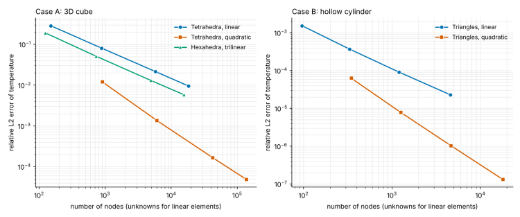
Figure 5. Relative L2 error against number of nodes.

For smooth problems like these, quadratic elements are the better choice. For problems with singularities or discontinuities the advantage shrinks, so this conclusion should not be extended without checking.

6. Does a parallel run give the same answer?

We also ran one mesh of each case on 4 MPI processes, with the mesh split by ElmerGrid using METIS (Karypis and Kumar). The relative L2 errors agree with the serial runs to seven digits:

Case	Mesh	Serial	4 MPI processes
A	quadratic tetrahedra, 8 divisions	1.353532e-03	1.353532e-03
B	quadratic triangles, h = 0.05	1.024297e-06	1.024297e-06

Case B was first solved with a direct solver (UMFPACK), which Elmer cannot use in parallel. We switched to conjugate gradients with ILU1 and confirmed that all serial errors stayed identical to four digits.

7. What this does not show

• No experimental validation. Exact solutions verify the numerics, not the physics.
• Steady, linear, smooth problems only. Temperature-dependent conductivity, transient behaviour, radiation, singularities and coupled physics are not covered.
• One run per mesh, with our own error code. Its credibility rests on the fact that the observed orders match theory in all five series.
• A local compilation. The results come from a local Elmer 9.0 compilation, not from the cloudHPC image. They are expected to match, but this has not been checked yet.
• Small parallel test. The parallel check used 4 processes on small meshes. It says nothing about scalability.

8. Next: Elmer on cloudHPC, and scalability

The next step is to repeat these cases on the elmerSolver-9.0 solver available on cloudHPC, and to add a strong-scaling test of Case A on a mesh with millions of elements. Published results from the Elmer team (CSC, PARA2012 tutorial) report a Poisson problem with 100 million unknowns solved on up to 2,176 cores, and suggest about 10⁴ unknowns per partition as a lower limit for good scaling. We will test how well that guideline holds on cloudHPC machines and add the results to this post.

References

1. Oberkampf, W. L. and Roy, C. J. Verification and Validation in Scientific Computing. Cambridge University Press, 2010. DOI: 10.1017/CBO9780511760396.
2. ASME V&V 20-2009. Standard for Verification and Validation in Computational Fluid Dynamics and Heat Transfer. American Society of Mechanical Engineers.
3. Roache, P. J. Code verification by the method of manufactured solutions. Journal of Fluids Engineering 124(1), 4-10, 2002.
4. Salari, K. and Knupp, P. Code verification by the method of manufactured solutions. Sandia National Laboratories report SAND2000-1444, 2000. Sandia publication page.
5. Incropera, F. P., DeWitt, D. P., Bergman, T. L. and Lavine, A. S. Fundamentals of Heat and Mass Transfer. Wiley (radial conduction in cylinders; any edition).
6. Carslaw, H. S. and Jaeger, J. C. Conduction of Heat in Solids, 2nd ed. Oxford University Press, 1959.
7. CSC – IT Center for Science. Elmer FEM, ElmerSolver Manual and Elmer Models Manual. elmerfem.org; source code: github.com/ElmerCSC/elmerfem, tag release-9.0.
8. ElmerTeam, CSC. Elmer scaling, PARA2012 tutorial, Helsinki, 2012. PDF.
9. Geuzaine, C. and Remacle, J.-F. Gmsh: a three-dimensional finite element mesh generator with built-in pre- and post-processing facilities. International Journal for Numerical Methods in Engineering 79(11), 1309-1331, 2009.
10. Karypis, G. and Kumar, V. A fast and high quality multilevel scheme for partitioning irregular graphs. SIAM Journal on Scientific Computing 20(1), 359-392, 1998.

---

CloudHPC is a HPC provider to run engineering simulations on the cloud. CloudHPC provides from 1 to 224 vCPUs for each process in several configuration of HPC infrastructure - both multi-thread and multi-core. Current software ranges includes several CAE, CFD, FEA, FEM software among which OpenFOAM, FDS, Blender and several others.

New users benefit of a FREE trial of 300 vCPU/Hours to be used on the platform in order to test the platform, all each features and verify if it is suitable for their needs

---

Contact Name/Surname *

Company Name *

Company address *

City *

State/Province *

Country *CountryArubaAfghanistanAngolaAnguillaÅland IslandsAlbaniaAndorraUnited Arab EmiratesArgentinaArmeniaAmerican SamoaAntarcticaFrench Southern TerritoriesAntigua and BarbudaAustraliaAustriaAzerbaijanBurundiBelgiumBeninBonaire, Sint Eustatius and SabaBurkina FasoBangladeshBulgariaBahrainBahamasBosnia and HerzegovinaSaint BarthélemyBelarusBelizeBermudaBolivia, Plurinational State ofBrazilBarbadosBrunei DarussalamBhutanBouvet IslandBotswanaCentral African RepublicCanadaCocos (Keeling) IslandsSwitzerlandChileChinaCôte d'IvoireCameroonCongo, The Democratic Republic of theCongoCook IslandsColombiaComorosCabo VerdeCosta RicaCubaCuraçaoChristmas IslandCayman IslandsCyprusCzechiaGermanyDjiboutiDominicaDenmarkDominican RepublicAlgeriaEcuadorEgyptEritreaWestern SaharaSpainEstoniaEthiopiaFinlandFijiFalkland Islands (Malvinas)FranceFaroe IslandsMicronesia, Federated States ofGabonUnited KingdomGeorgiaGuernseyGhanaGibraltarGuineaGuadeloupeGambiaGuinea-BissauEquatorial GuineaGreeceGrenadaGreenlandGuatemalaFrench GuianaGuamGuyanaHong KongHeard Island and McDonald IslandsHondurasCroatiaHaitiHungaryIndonesiaIsle of ManIndiaBritish Indian Ocean TerritoryIrelandIran, Islamic Republic ofIraqIcelandIsraelItalyJamaicaJerseyJordanJapanKazakhstanKenyaKyrgyzstanCambodiaKiribatiSaint Kitts and NevisKorea, Republic ofKuwaitLao People's Democratic RepublicLebanonLiberiaLibyaSaint LuciaLiechtensteinSri LankaLesothoLithuaniaLuxembourgLatviaMacaoSaint Martin (French part)MoroccoMonacoMoldova, Republic ofMadagascarMaldivesMexicoMarshall IslandsNorth MacedoniaMaliMaltaMyanmarMontenegroMongoliaNorthern Mariana IslandsMozambiqueMauritaniaMontserratMartiniqueMauritiusMalawiMalaysiaMayotteNamibiaNew CaledoniaNigerNorfolk IslandNigeriaNicaraguaNiueNetherlandsNorwayNepalNauruNew ZealandOmanPakistanPanamaPitcairnPeruPhilippinesPalauPapua New GuineaPolandPuerto RicoKorea, Democratic People's Republic ofPortugalParaguayPalestine, State ofFrench PolynesiaQatarRéunionRomaniaRussian FederationRwandaSaudi ArabiaSudanSenegalSingaporeSouth Georgia and the South Sandwich IslandsSaint Helena, Ascension and Tristan da CunhaSvalbard and Jan MayenSolomon IslandsSierra LeoneEl SalvadorSan MarinoSomaliaSaint Pierre and MiquelonSerbiaSouth SudanSao Tome and PrincipeSurinameSlovakiaSloveniaSwedenEswatiniSint Maarten (Dutch part)SeychellesSyrian Arab RepublicTurks and Caicos IslandsChadTogoThailandTajikistanTokelauTurkmenistanTimor-LesteTongaTrinidad and TobagoTunisiaTürkiyeTuvaluTaiwan, Province of ChinaTanzania, United Republic ofUgandaUkraineUnited States Minor Outlying IslandsUruguayUnited StatesUzbekistanHoly See (Vatican City State)Saint Vincent and the GrenadinesVenezuela, Bolivarian Republic ofVirgin Islands, BritishVirgin Islands, U.S.Viet NamVanuatuWallis and FutunaSamoaYemenSouth AfricaZambiaZimbabwe

Email *

Email

Confirm Email

Privacy *

• I accept the privacy conditions

Privacy Policy

Message

Send registration