Scaling a 20.7M-cell LES of flow past a cylinder (Re = 3900) with code_saturne on cloudHPC

Short version. We built a 20.7-million-cell large-eddy simulation (LES) of the flow past a circular cylinder at Re = 3900, ran it with code_saturne 9.0.1 on six cloudHPC configurations (32, 48 and 96 cores on hypercore; 32, 48 and 112 cores on highcore) and repeated every configuration with two mesh partitioners. The twelve runs gave three results that matter for anyone running large meshes in the cloud:

1. The default graph partitioner (PT-SCOTCH) is the bottleneck at high core counts. Mesh preprocessing took 13 min on 32 cores, but 3.2 hours on 96 hypercore cores and 2.1 hours on 112 highcore cores, almost entirely partitioning. A space-filling-curve partitioner (Hilbert) did the same job in 8–20 s.
2. The graph partitioner still gives faster time steps. The Hilbert partition makes each time step 8–27% longer, depending on the core count, because its halos are larger and less even. The gap grows with the core count, and the long SCOTCH preprocessing pays off after a few thousand time steps (about 26,000 steps on 96 hypercore cores, where its partitioning is slowest).
3. hypercore beats highcore for this case. At the same core count a time step is 2.5–2.7× faster on hypercore. Even though hypercore costs 0.11 € per core-hour against 0.05 € for highcore, a hypercore run is cheaper per time step and much faster. In the extreme case, 32 hypercore cores match the time per step of 112 highcore cores.

All numbers below are measured. The runs cover the performance side only: 400 time steps (one convective time unit) each, which is not long enough to compute shedding frequency or drag statistics. Section 7 explains what is and what is not established about the physics.

1. The test case

Flow past a circular cylinder at Re = U∞D/ν = 3900 is a standard LES benchmark. The wake is already turbulent, with a transitional shear layer, and experiments and simulations are well documented (Norberg 2003; Kravchenko & Moin 2000; Parnaudeau et al. 2008; Lehmkuhl et al. 2013). It is therefore a good case for stressing a CFD code: it is simple to describe, needs a fine mesh, and has a lot of literature to compare with.

Item	Value
Solver	code_saturne 9.0.1 (codeSaturne-9.0.1 on cloudHPC)
Turbulence model	LES with the WALE subgrid-scale model (Nicoud & Ducros 1999)
Reynolds number	3900 (ρ = 1, U = 1, D = 1, μ = 1/3900)
Time step	constant, Δt = 0.0025 D/U (400 steps = 1 convective time unit)
Mesh	structured O-grid, 720 (circumferential) × 240 (radial) × 120 (spanwise) = 20,736,000 hexahedra, 20,995,920 vertices
Domain	outer radius 15 D, spanwise length πD with periodic boundaries
Near-wall resolution	first cell height 0.003 D, radial growth ratio 1.0191, wall arc length 0.0044 D, spanwise Δz = 0.026 D
Boundaries	inlet U = (1, 0, 0) on the upstream half of the outer circle, free outlet on the downstream half, smooth no-slip cylinder, translation periodicity in z
Convection scheme	blending factor 1.0 (centred) for velocity, 10 and 5 reconstruction sweeps for velocity and pressure (the values code_saturne recommends for LES)
Output	cylinder force history and four velocity probes every step; no volume output during the scaling runs

Figure 1. The O-grid. Left: the full domain (R = 15 D, every 12th ring shown). Right: detail around the cylinder (every 2nd ring shown).

Building a 20-million-cell mesh in the cloud

The mesh is generated by a short Python script (numpy and scipy) that writes a Gmsh MSH 2.2 binary file layer by layer along the span, so memory stays small even for 20M cells. A few practical details worth knowing if you reproduce this:

• code_saturne reads Gmsh MSH. With the version 2 format, groups are identified by the numeric physical tag, so selection criteria in cs_user_zones and cs_user_mesh must use "1", "2"… rather than names such as cylinder. (Physical names are only honoured in version 4.) Our first smoke test failed on exactly this point.
• The spanwise periodicity is defined in cs_user_mesh with a translation of πD between the two lateral faces (criterion "4 or 5").
• The mesh file is 1.5 GB (517 MB compressed). Instead of uploading it from a laptop, we generated the case on a cloudHPC machine: a small custom-script-u24 job (8 vCPU, about €0.05) ran the generator and pushed the compressed case straight into the six storage folders through pre-signed upload links. The whole generation and distribution took about ten minutes.

2. Test matrix and hardware

code_saturne runs one MPI process per physical core. On cloudHPC the highcore and hypercore families give physical cores only (hypercore uses a newer CPU generation). We used three sizes per family and two partitioners, in separate storage folders, for 12 runs in total.

Family	Cores	CPU that cloudHPC assigned	Price
hypercore	32	Intel Xeon Platinum 8581C	0.11 €/core-h
hypercore	48	AMD EPYC 9B45	0.11 €/core-h
hypercore	96	AMD EPYC 9B45	0.11 €/core-h
highcore	32, 48, 112	AMD EPYC 7B13	0.05 €/core-h

The CPU model was read from the log of each run, except for the SCOTCH runs on 96 hypercore and 112 highcore cores, where it is the model that cloudHPC assigned to the same configuration in the Hilbert run.

Two caveats come with this table, and they shape how the results should be read:

• The hypercore family mixes two CPU types. The 32-core run landed on an Intel machine, while the 48- and 96-core runs landed on AMD EPYC 9B45. The speed-up of hypercore therefore combines core count and CPU change, and we did not measure the single-core speed of each CPU. The highcore family is clean: all runs used the same AMD EPYC 7B13.
• All machines were preemptible (the default on cloudHPC). One run (highcore 32, Hilbert) was preempted once, restarted automatically from the beginning, and completed. Its wall-clock time and cost include the lost work, but its per-step timing is unaffected.

3. Method

• Time per step is measured inside the solver (cs_timer_wtime() at each step, written by a small user routine to a history file), so it excludes preprocessing, I/O and VM start-up. We discard the first 50 steps and average steps 51–400. Uncertainty is the standard error over seven blocks of 50 steps, and it is reported in the CSV file attached to this post.
• Speed-up is the time per step of the smallest run (32 cores) divided by the time per step of the larger run, within the same family and with the same partitioner. Efficiency is the speed-up divided by the ideal speed-up (cores / 32).
• Preprocessing is the “Total elapsed time for preprocessing” line of code_saturne’s performance.log: mesh reading, partitioning, joining of the periodic faces and renumbering.
• Cost is the amount billed by cloudHPC for each run, as returned by the platform. It includes the VM start-up, preprocessing, I/O and result upload, not only the 400 steps.
• Each configuration was run once, so there is no run-to-run repetition. The standard errors above describe the noise between steps inside a run, not the variability between runs.

4. Results

Figure 2. Mesh preprocessing time (log scale). With PT-SCOTCH, preprocessing grows from 13–15 min at 32 cores to 3.2 h at 96 hypercore cores and 2.1 h at 112 highcore cores. With the Hilbert curve it stays between 8 and 20 s.

4.1 Partitioning is where the default breaks down

During preprocessing, code_saturne first splits the cells with a fast Morton curve, then performs the join of the periodic faces, then re-partitions with PT-SCOTCH. In the logs, the PT-SCOTCH step alone took 772 s on 32 hypercore cores and 1.16 × 10⁴ s on 96. During that phase the machine’s CPU traces show one or two cores busy and the rest idle, so a 96-core instance (€10.56/h) spends hours doing serial work. The 96-core SCOTCH run cost €37.62, nine times the €4.13 of the same run with the Hilbert partitioner, for a result that differs only in the partition.

4.2 The graph partitioner gives faster steps

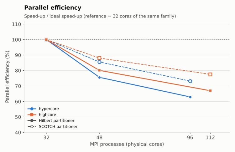
Figure 3. Time per step (steps 51–400, error bars are the standard error of seven blocks). Solid lines: Hilbert partitioner. Dashed lines: PT-SCOTCH.

Once the mesh is partitioned, the PT-SCOTCH partition runs faster. The Hilbert time per step is 8–10% higher at 32 cores, 21–22% higher at 48 cores and 25–27% higher at 96/112 cores. The logs show why. The Hilbert curve balances the number of cells perfectly (every rank gets exactly the same count), but the partitions are less compact. The largest number of cells per rank including halo cells (the ghost layer exchanged at every step) is higher than with SCOTCH, and the gap tracks the time penalty:

Config	Max cells + halo per rank, SCOTCH	Max cells + halo per rank, Hilbert	Hilbert / SCOTCH	Time per step, Hilbert / SCOTCH
hypercore 32	703,695	746,992	1.06	1.08
hypercore 48	479,798	546,636	1.14	1.22
hypercore 96	250,126	289,300	1.16	1.25
highcore 32	705,467	746,992	1.06	1.10
highcore 48	483,811	546,636	1.13	1.21
highcore 112	216,374	271,006	1.25	1.27

The most loaded rank sets the pace of every step, so a larger and more uneven halo on that rank costs time. We did not instrument the MPI communication directly, so this is a consistent explanation rather than a proven one.

4.3 Scalability

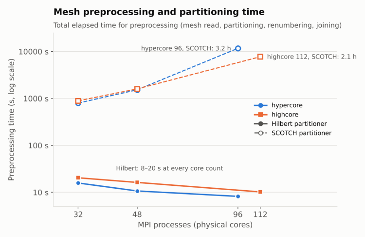
Figure 4. Speed-up against the 32-core run of the same family and partitioner.

Figure 5. Parallel efficiency.

The full table follows (the CSV with the standard errors and the CPU type is attached).

Family	Cores	Cells/core	Partitioner	Time/step (s)	Speed-up	Efficiency	Preproc. (s)	Run cost (€)	Run ID
hypercore	32	648 k	SCOTCH	3.85	1.00	100%	797	2.91	89812
hypercore	32	648 k	Hilbert	4.16	1.00	100%	16	2.31	89836
hypercore	48	432 k	SCOTCH	3.00	1.28	86%	1527	4.59	89825
hypercore	48	432 k	Hilbert	3.67	1.13	76%	11	2.79	89837
hypercore	96	216 k	SCOTCH	1.75	2.20	73%	11653	37.62	89818
hypercore	96	216 k	Hilbert	2.20	1.89	63%	8	4.13	89838
highcore	32	648 k	SCOTCH	10.20	1.00	100%	889	2.44	89819
highcore	32	648 k	Hilbert	11.20	1.00	100%	20	2.43	89839
highcore	48	432 k	SCOTCH	7.72	1.32	88%	1596	3.51	89820
highcore	48	432 k	Hilbert	9.32	1.20	80%	16	2.82	89840
highcore	112	185 k	SCOTCH	3.76	2.71	78%	7725	15.60	89821
highcore	112	185 k	Hilbert	4.78	2.34	67%	10	3.75	89841

Reading the table:

• Highcore is the cleaner scaling test (same CPU everywhere). With SCOTCH, efficiency is 88% at 48 cores and 78% at 112 cores. With Hilbert it is 80% and 67%. For a 20.7M-cell mesh, 185,000 cells per core is already in the regime where communication costs show.
• Hypercore efficiency is confounded by the CPU change between 32 and 48 cores, as explained in section 2. If the AMD cores are faster per core than the Intel ones, the true efficiency at 48 and 96 cores is lower than the 86% and 73% shown. We can only say that scalability is no better than that.
• Absolute speed. At equal core counts, a hypercore step takes 2.5–2.7× less than a highcore step (3.85 s against 10.20 s at 32 cores with SCOTCH). The 32-core hypercore run (3.85 s/step) is as fast as the 112-core highcore run (3.76 s/step).

Rule of thumb: cells per core. For code_saturne with LES on hexahedral meshes, on this kind of machine, keep at least 200–250k cells per core.

Cells per core	Measured efficiency (SCOTCH, vs 648k cells/core)
~430k	86–88%
~215k (hypercore 96)	73%
~185k (highcore 112)	78%

Above 400k cells per core, efficiency stays above 85%. Below 200k you already lose about a quarter of the cores you pay for. With the Hilbert partitioner the loss is larger: 63–67% efficiency at 185–215k cells per core.

Limits of this rule: our data do not go below 185k cells per core, so we cannot say where the curve collapses. It comes from one case (LES, WALE model, 20.7M hexahedra), one run per configuration, and we have not compared it with published scaling studies. A different turbulence model or additional physics will shift the threshold. If your case has fewer cells per core than this, use fewer cores or a finer mesh.

Figure 6. Cost of each 400-step run, including preprocessing, I/O and VM start-up.

4.4 What this means for a production run

The 400-step runs are dominated by fixed costs, so they are not the right basis to choose a configuration for a long simulation. The table below projects the compute-only cost of 100,000 time steps (about 250 convective time units at Δt = 0.0025) from the measured time per step and the observed prices. It is an extrapolation, assuming the time per step stays constant, and it excludes preprocessing and I/O.

Config	Partitioner	Wall-clock for 100k steps	Compute cost
hypercore 32	SCOTCH	107 h	€ 377
hypercore 48	SCOTCH	83 h	€ 441
hypercore 96	SCOTCH	49 h	€ 515
hypercore 96	Hilbert	61 h	€ 646
highcore 32	SCOTCH	283 h	€ 454
highcore 112	SCOTCH	104 h	€ 585
highcore 112	Hilbert	133 h	€ 743

Three practical conclusions follow:

1. For short runs and for tests, use the Hilbert partitioner. Up to a few thousand steps, the time saved on preprocessing beats the slower steps. The break-even between the two partitioners, computed from our data, is about 900–1,000 steps on 32–48 highcore cores, about 2,300–2,600 steps on 32–48 hypercore cores, 7,600 steps on 112 highcore cores and 26,000 steps on 96 hypercore cores.
2. For a long production run, the SCOTCH partition is worth having, because its time steps are 17–21% shorter at 48 cores and above (the Hilbert steps take 21–27% longer). The problem is paying for the partitioning on an expensive machine. code_saturne can write the partition to a partition_output folder and read it back from partition_input in a later run (the log of each run checks for partition_input/domain_number_N), so the cleanest approach is to compute the partition once and reuse it. We have not tested this workflow here, so treat it as the next experiment, not as a result.
3. Prefer hypercore over highcore for this solver and mesh. It is faster per step and cheaper per step at the same core count. For example, 100,000 steps on 32 hypercore cores cost about €377 against about €454 on 32 highcore cores, in less than half the wall-clock time. Highcore only wins on the price per core-hour, not on the price per result.

5. What we learned about running code_saturne on cloudHPC

• User C++ sources placed in SRC/ are compiled automatically, and setup.xml is picked up from DATA/. A case with a custom cs_user_mesh.cpp, cs_user_zones.cpp and cs_user_performance_tuning.cpp needs no other setup.
• Changing the partitioner takes seven lines in cs_user_performance_tuning.cpp:

cpp

void
cs_user_partition(void)
{
  cs_partition_set_algorithm(CS_PARTITION_MAIN,
                             CS_PARTITION_SFC_HILBERT_BOX,
                             1,       /* rank_step */
                             false);  /* ignore periodicity in graph */
}

• The result archive of a 20M-cell run is about 2.9 GB, mostly the intermediate mesh files (mesh_input.csm, mesh_output.csm). To keep only the logs and histories, stream-extract the archive and exclude *.csm, the checkpoint and the postprocessing folders.
• Instances in one zone can run out. Our runs were automatically moved to another zone of the same region when the first was out of stock, which can change the CPU type, as noted in section 2.

6. Limitations of this scaling study

• One run per configuration and no repetition between runs.
• Hypercore results mix two CPU types (section 2).
• Only 400 time steps per run: start-up costs such as the first linear-solver solves are excluded by discarding 50 steps, but any slow change of the cost per step as the wake develops is not captured.
• Time per step depends on the number of iterations of the pressure solver, which changes with the flow state. A fully developed wake may cost somewhat more or less per step than the start-up we measured.
• The scalability numbers refer to this mesh (20.7M cells) and this solver set-up. A bigger mesh scales further, a smaller one does not.

7. About the physics: what is and what is not established

The scaling runs were configured for performance measurements, so they are not a validation of the LES. The force history of the first convective time unit shows why.

Figure 7. Drag and lift coefficients over the 400 steps of the hypercore 32 Hilbert run. The impulsive start produces a very large spike at step 2 (Cd ≈ 630, off scale) and a step-to-step oscillation in the force that has not yet decayed after one convective unit.

The solution starts impulsively from a uniform flow with a small perturbation. In such a start-up, the pressure force on the wall oscillates from one step to the next. The amplitude decays at first, then grows again at the end of the run, so we cannot say whether this oscillation damps out in a long run or points to a set-up issue. It does not affect the performance results (the cost of a step is the same), but it means we make no claim about drag, Strouhal number or wake statistics from these runs.

The quantities to compare against the benchmark literature (Strouhal number near 0.2, mean drag coefficient near 1, mean velocity profiles and Reynolds stresses in the near wake; Kravchenko & Moin 2000; Parnaudeau et al. 2008; Norberg 2003) need a much longer run, with time-averaged profiles collected after the transient. The mesh has 0.026 D spanwise spacing and 0.0044 D circumferential spacing at the wall, but mesh resolution alone does not validate a simulation. The natural follow-up is a run of about 100 convective time units on the best configuration (96 hypercore cores with the SCOTCH partition: about 40,000 steps, roughly 20 hours at the measured 1.75 s per step), with time-averaged profiles collected after the transient.

8. Reproducing this on cloudHPC

1. Generate the mesh and the case (we used a custom-script-u24 job to do it in the cloud).
2. Put the case (DATA/, SRC/, MESH/) in a storage folder.
3. Launch codeSaturne-9.0.1 on the number of cores you want, on hypercore or highcore.
4. Read the time per step from the history file written by the user routine, and the preprocessing time from performance.log.

All twelve launches, the monitoring and the result downloads of this study were driven from an AI assistant through the cloudHPC MCP server, which exposes the same operations as the web interface.

References

The following sources were consulted and checked while preparing this study. Journal references were checked against the publisher, library or repository record, except where noted.

Test case and LES literature

• Kravchenko, A. G., & Moin, P. (2000). Numerical studies of flow over a circular cylinder at Re_D = 3900. Physics of Fluids, 12(2), 403–417. doi:10.1063/1.870318
• Parnaudeau, P., Carlier, J., Heitz, D., & Lamballais, E. (2008). Experimental and numerical studies of the flow over a circular cylinder at Reynolds number 3900. Physics of Fluids, 20(8), 085101. doi:10.1063/1.2957018– Lehmkuhl, O., Rodríguez, I., Borrell, R., & Oliva, A. (2013). Low-frequency unsteadiness in the vortex formation region of a circular cylinder. Physics of Fluids, 25(8). doi:10.1063/1.4818641. Repository record: recercat.cat/handle/2072/223671
• Norberg, C. (2003). Fluctuating lift on a circular cylinder: review and new measurements. Journal of Fluids and Structures, 17(1), 57–96. doi:10.1016/S0889-9746(02)00099-3. Record: lup.lub.lu.se/record/317278
• Nicoud, F., & Ducros, F. (1999). Subgrid-scale stress modelling based on the square of the velocity gradient tensor. Flow, Turbulence and Combustion, 62, 183–200. doi:10.1023/A:1009995426001

Software and numerical methods

• Archambeau, F., Méchitoua, N., & Sakiz, M. (2004). Code_Saturne: a finite volume code for the computation of turbulent incompressible flows – industrial applications. International Journal on Finite Volumes, 1(1). ijfv.math.cnrs.fr
• code_saturne 9.0.1 source and release: github.com/code-saturne/code_saturne, tag v9.0.1
• code_saturne 9.0 documentation, cs_user_performance_tuning (advanced partitioning, cs_partition_set_algorithm, Morton and Hilbert curves, SCOTCH, METIS): code-saturne.org/documentation/9.0/doxygen/src/cs_user_performance_tuning.html
• code_saturne user example cs_user_performance_tuning-partition.cpp (tag v9.0.1) used as the model for our cs_user_partition: raw.githubusercontent.com/code-saturne/code_saturne/v9.0.1/src/user_examples/cs_user_performance_tuning-partition.cpp
• Pellegrini, F., & Roman, J. (1996). SCOTCH: a software package for static mapping by dual recursive bipartitioning of process and architecture graphs. Lecture Notes in Computer Science, vol. 1067, p. 493 ff. (HPCN Europe 1996). Bibliographic record: ftp.math.utah.edu/pub/tex/bib/idx/lncs1996a/1067/0/493-z.html (end page not given in the record).
• Geuzaine, C., & Remacle, J.-F. (2009). Gmsh: a three-dimensional finite element mesh generator with built-in pre- and post-processing facilities. International Journal for Numerical Methods in Engineering, 79(11), 1309–1331. As requested for citation on gmsh.info. MSH format documentation: gmsh.info/doc/texinfo/gmsh.html (section 10.3.1, MSH file format version 2).

---

CloudHPC is a HPC provider to run engineering simulations on the cloud. CloudHPC provides from 1 to 224 vCPUs for each process in several configuration of HPC infrastructure - both multi-thread and multi-core. Current software ranges includes several CAE, CFD, FEA, FEM software among which OpenFOAM, FDS, Blender and several others.

New users benefit of a FREE trial of 300 vCPU/Hours to be used on the platform in order to test the platform, all each features and verify if it is suitable for their needs

---

Contact Name/Surname *

Company Name *

Company address *

City *

State/Province *

Country *CountryArubaAfghanistanAngolaAnguillaÅland IslandsAlbaniaAndorraUnited Arab EmiratesArgentinaArmeniaAmerican SamoaAntarcticaFrench Southern TerritoriesAntigua and BarbudaAustraliaAustriaAzerbaijanBurundiBelgiumBeninBonaire, Sint Eustatius and SabaBurkina FasoBangladeshBulgariaBahrainBahamasBosnia and HerzegovinaSaint BarthélemyBelarusBelizeBermudaBolivia, Plurinational State ofBrazilBarbadosBrunei DarussalamBhutanBouvet IslandBotswanaCentral African RepublicCanadaCocos (Keeling) IslandsSwitzerlandChileChinaCôte d'IvoireCameroonCongo, The Democratic Republic of theCongoCook IslandsColombiaComorosCabo VerdeCosta RicaCubaCuraçaoChristmas IslandCayman IslandsCyprusCzechiaGermanyDjiboutiDominicaDenmarkDominican RepublicAlgeriaEcuadorEgyptEritreaWestern SaharaSpainEstoniaEthiopiaFinlandFijiFalkland Islands (Malvinas)FranceFaroe IslandsMicronesia, Federated States ofGabonUnited KingdomGeorgiaGuernseyGhanaGibraltarGuineaGuadeloupeGambiaGuinea-BissauEquatorial GuineaGreeceGrenadaGreenlandGuatemalaFrench GuianaGuamGuyanaHong KongHeard Island and McDonald IslandsHondurasCroatiaHaitiHungaryIndonesiaIsle of ManIndiaBritish Indian Ocean TerritoryIrelandIran, Islamic Republic ofIraqIcelandIsraelItalyJamaicaJerseyJordanJapanKazakhstanKenyaKyrgyzstanCambodiaKiribatiSaint Kitts and NevisKorea, Republic ofKuwaitLao People's Democratic RepublicLebanonLiberiaLibyaSaint LuciaLiechtensteinSri LankaLesothoLithuaniaLuxembourgLatviaMacaoSaint Martin (French part)MoroccoMonacoMoldova, Republic ofMadagascarMaldivesMexicoMarshall IslandsNorth MacedoniaMaliMaltaMyanmarMontenegroMongoliaNorthern Mariana IslandsMozambiqueMauritaniaMontserratMartiniqueMauritiusMalawiMalaysiaMayotteNamibiaNew CaledoniaNigerNorfolk IslandNigeriaNicaraguaNiueNetherlandsNorwayNepalNauruNew ZealandOmanPakistanPanamaPitcairnPeruPhilippinesPalauPapua New GuineaPolandPuerto RicoKorea, Democratic People's Republic ofPortugalParaguayPalestine, State ofFrench PolynesiaQatarRéunionRomaniaRussian FederationRwandaSaudi ArabiaSudanSenegalSingaporeSouth Georgia and the South Sandwich IslandsSaint Helena, Ascension and Tristan da CunhaSvalbard and Jan MayenSolomon IslandsSierra LeoneEl SalvadorSan MarinoSomaliaSaint Pierre and MiquelonSerbiaSouth SudanSao Tome and PrincipeSurinameSlovakiaSloveniaSwedenEswatiniSint Maarten (Dutch part)SeychellesSyrian Arab RepublicTurks and Caicos IslandsChadTogoThailandTajikistanTokelauTurkmenistanTimor-LesteTongaTrinidad and TobagoTunisiaTürkiyeTuvaluTaiwan, Province of ChinaTanzania, United Republic ofUgandaUkraineUnited States Minor Outlying IslandsUruguayUnited StatesUzbekistanHoly See (Vatican City State)Saint Vincent and the GrenadinesVenezuela, Bolivarian Republic ofVirgin Islands, BritishVirgin Islands, U.S.Viet NamVanuatuWallis and FutunaSamoaYemenSouth AfricaZambiaZimbabwe

Email *

Email

Confirm Email

Privacy *

• I accept the privacy conditions

Privacy Policy

Website

Send registration