DAFoam: Let the Adjoint Design Your Shape
The classic design loop in CFD goes like this: guess a shape, mesh it, simulate it, look at the result, tweak the geometry, repeat. It works when a design has three or four parameters. It stops working when the shape is described by dozens or hundreds of variables, because nobody can explore that space by hand, and brute-force sampling costs one simulation per variable just to learn which way to move.
DAFoam takes a different route. Instead of asking “what happens if I change this?”, it asks the flow solver directly for the gradient of the quantity you care about with respect to every design variable at once, and lets an optimizer follow it. This post explains what DAFoam is, why the adjoint method makes this affordable, and walks through a complete airfoil optimization that ran on cloudHPC in a few minutes. The case files are free to download at the end.
What DAFoam is
DAFoam (Discrete Adjoint with OpenFOAM) is an open-source framework for high-fidelity, gradient-based design optimization built on top of OpenFOAM. It was developed by Ping He and co-authors at the University of Michigan’s MDO Lab and is now led by his group at Iowa State University. It adds to OpenFOAM what OpenFOAM does not have by itself: the ability to compute exact sensitivities of an objective with respect to shape and flow parameters, and a Python interface that plugs those sensitivities into an optimizer.
In practice, a DAFoam case looks like an ordinary OpenFOAM case (0/, constant/, system/) plus a Python run script that defines the objective, the constraints and the design variables. The optimization is orchestrated through OpenMDAO and MPhys, and the optimizer itself comes from pyOptSparse (SLSQP, IPOPT, SNOPT and others).
Why the adjoint matters
This is the idea that makes the whole approach work.
Suppose the drag of an airfoil depends on 100 shape variables. To estimate the gradient with finite differences, you perturb each variable in turn and rerun the flow: 100 extra simulations for one gradient, and you need a new gradient at every optimization step.
The adjoint method gets the same gradient by solving one additional linear system per function of interest, whatever the number of design variables. Drag with respect to 10 variables or 1,000 variables costs essentially the same: one flow solve plus one adjoint solve. If lift is also a constraint, add one more adjoint solve for lift. The cost scales with the number of objectives and constraints, not with the number of design variables.
That is what turns detailed shape optimization from a research exercise into something you can run on a normal budget. DAFoam implements the discrete adjoint, which means the gradients are consistent with the discretized equations the solver actually uses, so the optimizer gets derivatives it can trust.
What it can do
- Incompressible and compressible steady flows, with the standard RANS turbulence models
- Heat transfer and conjugate heat transfer problems
- Turbomachinery, with a mixing-plane setup ready for optimization
- Free-form deformation (FFD) shape parameterization, plus flow variables such as the angle of attack as design variables
- Geometric constraints: thickness, volume, leading-edge radius and more
- Coupling to pyOptSparse optimizers through OpenMDAO
- User-defined objectives, for example efficiency or pressure loss instead of drag
Example: minimizing the drag of a NACA0012 at constant lift
To show the whole workflow end to end, we took the official DAFoam NACA0012 tutorial and ran it on cloudHPC with the pre-installed DAFoam v5.0.0 image (OpenFOAM v2506).
The problem. A 2D NACA0012 airfoil with 1 m chord in a 10 m/s incompressible flow (Re ≈ 6.7×10⁵), Spalart-Allmaras turbulence model. The goal is to minimize the drag coefficient while keeping the lift coefficient at CL = 0.5. The optimizer controls 8 FFD shape variables plus the angle of attack. Three geometric constraints keep the result realistic: thickness at least 50% of the original at every station, total volume at least equal to the original, and leading-edge radius at least 80% of the original.
The workflow. A single Allrun script does everything: it generates the 4,032-cell mesh, trims the baseline airfoil to CL = 0.5, runs the optimization with SLSQP, and produces the plots and a summary table. The core of it is one line:
bash
mpirun -np 4 python runOptimization.py -task all -optimizer SLSQPThe objective and the lift constraint are defined in a few lines of the run script:
python
"function": {
    "CD": {"type": "force", "source": "patchToFace", "patches": ["wing"],
           "directionMode": "parallelToFlow", "patchVelocityInputName": "patchV",
           "scale": 1.0 / (0.5 * U0 * U0 * A0 * rho0)},
    "CL": {"type": "force", "source": "patchToFace", "patches": ["wing"],
           "directionMode": "normalToFlow", "patchVelocityInputName": "patchV",
           "scale": 1.0 / (0.5 * U0 * U0 * A0 * rho0)},
},
and the optimization problem in a few more:
python
self.add_design_var("shape", lower=-1.0, upper=1.0, scaler=10.0)
self.add_design_var("patchV", lower=[U0, 0.0], upper=[U0, 10.0], scaler=0.1)
self.add_objective("scenario1.aero_post.CD", scaler=1.0)
self.add_constraint("scenario1.aero_post.CL", equals=0.5, scaler=1.0)
self.add_constraint("geometry.thickcon", lower=0.5, upper=3.0, scaler=1.0)
self.add_constraint("geometry.volcon", lower=1.0, scaler=1.0)
self.add_constraint("geometry.rcon", lower=0.8, scaler=1.0)
Results
| CD | CL | Angle of attack | |
|---|---|---|---|
| Baseline NACA0012 | 0.020944 | 0.5000 | 5.15° |
| Optimized | 0.017657 | 0.5000 | 1.38° |
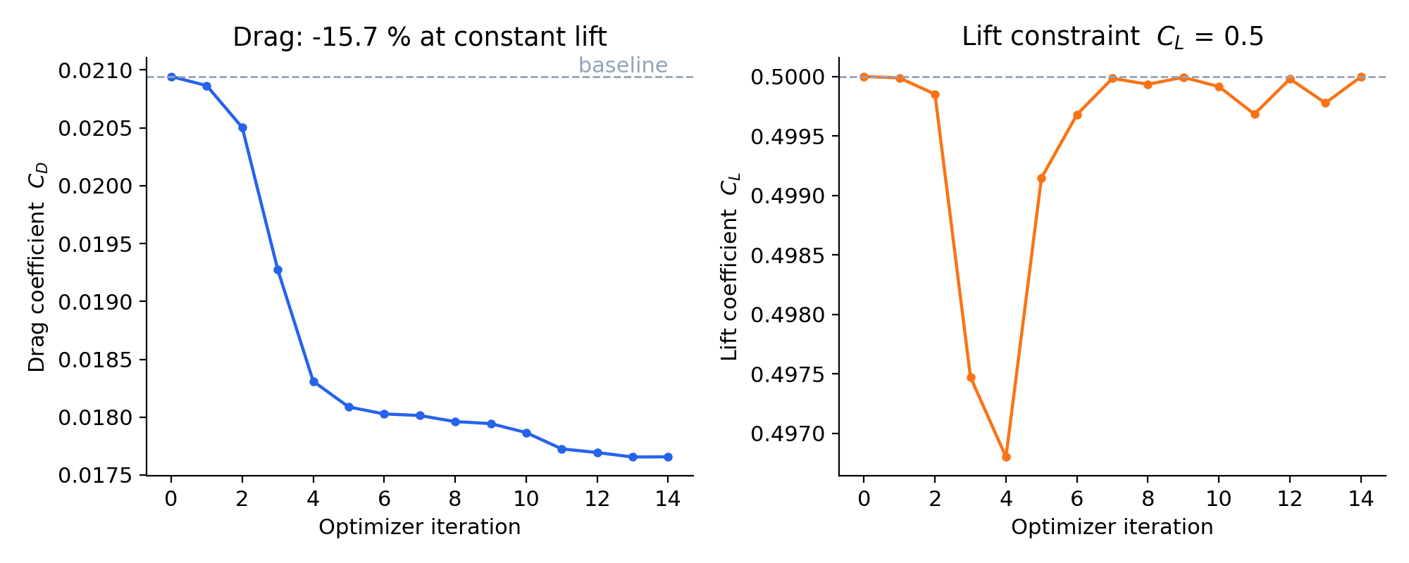
Drag drops by 15.7% at the same lift. SLSQP converged after 15 flow evaluations and 14 gradient evaluations, and every flow and adjoint solve converged to tight tolerances along the way.

Figure 1. Left: drag coefficient versus optimizer iteration; most of the gain arrives in the first four iterations, then the design settles. Right: lift coefficient. The dip around iteration 4 is the optimizer taking a large step in shape; it restores CL = 0.5 within a few iterations.

Figure 2. Top: baseline NACA0012 and optimized airfoil. Bottom: vertical displacement of the upper and lower surfaces along the chord.
Figure 2 shows what the optimizer found. Both surfaces moved upward by roughly 3% of the chord, so the thickness stays close to the original while the airfoil gains camber. A cambered airfoil produces the required lift at a much lower angle of attack (1.4° instead of 5.2°), which is where the drag saving comes from. At the optimum the volume and leading-edge-radius constraints are active: they are what stops the optimizer from going further.
A note on scope: the mesh is deliberately coarse so that the whole case runs in minutes, and it uses wall functions. Treat the absolute drag values as indicative. The comparison between baseline and optimized designs, computed with the same mesh and model, is the meaningful result, and the method is exactly the same one you would use on a production mesh.
How long did it take?
On a 4-core cloudHPC instance, the optimization loop itself took 141 seconds, of which 116 seconds were spent computing gradients. The full job, including mesh generation, the baseline trim and post-processing, finished in a few minutes of compute time and cost a few cents.
Why run DAFoam on cloudHPC
It is worth being precise about the shape of this workload, because it is different from a parameter sweep.
Adjoint optimization is sequential. Each design iteration needs a flow solve and then the adjoint solves, and the next iteration depends on the result. You cannot spread the iterations across many machines. What you can do is make each iteration fast, and that is where the platform matters:
- Right-sized nodes for each solve. DAFoam runs one MPI rank per physical core. On cloudHPC you pick the number of cores for the size of your mesh, from a 4-core instance for a 2D case like this one to large nodes for 3D production meshes.
- Memory for the adjoint. The adjoint needs noticeably more memory than the flow solve alone. Choosing an instance with enough RAM up front avoids the most common way these runs fail on a workstation.
- No queue between iterations. A job runs from the first flow solve to the last gradient on dedicated hardware, and you pay only for the time it runs.
- No build. DAFoam depends on OpenFOAM builds compiled with automatic differentiation plus a Python stack (PETSc, pyOptSparse, OpenMDAO, MPhys, pyGeo, IDWarp). Building all of this from source takes hours and is easy to get wrong. On cloudHPC, DAFoam v5.0.0 is pre-installed: upload the case, choose the solver, launch.
Try it yourself
Download the case used in this post: dafoam-naca0012-cloudhpc.zip
To run it on cloudHPC:
- Upload the zip to your cloudHPC storage.
- Launch it with the DAFoam-v5.0.0 solver on a 4-vCPU highcore instance.
- cloudHPC detects the
Allrunscript and runs the whole chain. When it finishes, thefigures/folder contains the same plots shown above andlog.runOptimizationends with the baseline vs optimized table.
The same case also runs in any local DAFoam v5 environment with ./Allrun. The README in the zip explains every step and lists the small changes made to the official tutorial.
From here, the natural next steps are changing the objective (for example maximizing lift-to-drag ratio), adding more FFD control points, or moving to a 3D wing. The workflow stays the same; only the mesh and the node size grow.
DAFoam is developed by Ping He and co-authors. Reference: P. He, C. A. Mader, J. R. R. A. Martins, K. J. Maki, “DAFoam: An open-source adjoint framework for multidisciplinary design optimization with OpenFOAM”, AIAA Journal 58:1304–1319, 2020, doi:10.2514/1.J058853. Documentation and tutorials: dafoam.github.io.
CloudHPC is a HPC provider to run engineering simulations on the cloud. CloudHPC provides from 1 to 224 vCPUs for each process in several configuration of HPC infrastructure - both multi-thread and multi-core. Current software ranges includes several CAE, CFD, FEA, FEM software among which OpenFOAM, FDS, Blender and several others.
New users benefit of a FREE trial of 300 vCPU/Hours to be used on the platform in order to test the platform, all each features and verify if it is suitable for their needs

